programming – Kevin Martin Jose

Lessons learned from making a SaaS* completely serverless**

April 7, 2023April 7, 2023 Kevin3 Comments

* Software as a Service

** serverless as in everything runs on AWS lambda.

Short summary

I recently launched TweetScreenr. Going completely serverless kept the cloud costs low during development. I used the serverless framework to deploy my python flask API end points as AWS lambda functions. However this slowed down the development speed and I ran into tricky issues and limitations.

The full story

I recently launched TweetScreenr, a service that would create a personalized news feed out of your Twitter timeline, and I decided to use a completely serverless stack.

Why I decided to go serverless

I decided to re-write my app as serverless in an effort to avoid issues I faced in the past with regular AWS EC2 instances. Skip this section if you do not care about my motivation behind switching to serverless. Summary – I thought it would be cheaper and will require less babysitting.

I had launched the same service (minus some nice features) under a different name a year ago. It was a regular python flask web app with sqlite as the database and rabbitMQ as the message broker. I wasn’t expecting much traffic, so everything – the dabatase, the message broker and the web server – was running on an AWS EC2 t2.micro. It had 2 vCPUs and 1 GB of RAM and costed around $5 a month. Needless to say, it couldn’t handle the traffic from being on the front-page of HN. This was expected. But instead of requests just taking longer or the service being temporarily unavailable, the EC2 instance just went into a failed state and required manual intervention to restore the service. This wasn’t expected. I was hoping that the t2.micro would become unresponsive in the face of overwhelming traffic and would become functional again as the traffic died down. I didn’t expect it to crash and require a manual restart.

What was happening was that my t2.micro instance was running out of CPU credits and was throttling to 5% of the CPU performance, which isn’t enough to run the kernel. Burstable instances provides a baseline CPU performance and has the ability to burst above this baseline when the workload demands it. You accumulate CPU credits when the CPU is running at the baseline level and you use up these credits when you are bursting. I didn’t know that using up all your CPU credits for the instance can prevent the kernel from running. Using a t2.small didn’t solve the issue – I eventually ran out of CPU credits and the instance failed and required a manual intervention. The need to intervene manually meant that if the service goes down in the middle of the night, it stays down until I wake up the next morning.

You can argue that I was using the wrong EC2 instance type for the job and you would be right. I chose a t2.micro because it was the cheapest. The cheapest non-burstable instance I could find was an a1.medium for $18 a month, or $11 a month if I reserve it for a year. For a side project that didn’t have a plan to charge its users (yet), I considered that expensive. I considered moving to a $5 linode, but I was worried I’d run into variants of the same issue. Given the choices, going serverless sounded like a good idea. Each request to my service will be executed in a different lambda function and hence won’t starve for resources, even when there is high traffic. Moreover, I would be paying only for the compute I use. I did some calculations and figured that I can probably stay under the limits of the AWS free tier. It took me around a year to re-write the app to be completely serverless, add some new features and a paid tier, and launch again on HN. This time, the app did not go down. But the post also didn’t make it to the front-page, so I do not know what will happen if it’s subjected to the same amount of traffic.

The serverless stack

I wanted to use python flask during development and deploy each API route as a different lambda function. I used the confusingly named serverless framework to do exactly that. The serverless framework is essentially a wrapper around a cloud provider (AWS in my case) and automates the annoying job of creating an AWS API gateway end-point for each of the API routes in your app. It also has a bunch of plugins to handle things like managing a domain name, using static s3 assets e.t.c.

I had to use dynamoDB. If I had gone with a relational database, I’d again have to decide where to host the database (eg: t2.micro?). Instead of self-hosting RabbitMQ, I decided to use AWS SQS because my usage would fit in the free tier and allows me to easily configure a lambda function to process messages in the queue. If I had self-hosted RabbitMQ I would have had to use something like celery to process messages added to the queue, and that would have been an additional headache.

The good

Costs were low

I was able to keep costs exceptionally low during development. I wanted to have separate test, dev and prod stages. All experimental features are tested on test, and then promoted to dev once they are stable enough. If nothing explodes in dev for a while, the changes get deployed to prod. This would have required 3 EC2 instances running round the clock. Even if I were to use t2.micros, it would have been $15 a month to keep all three running all the time. It costs $0 with my AWS + serverless framework setup. Costs continued to remain low (i.e zero) even after I launched. I currently have 8 active users (including me) and I’m yet to exceed the AWS free-tier.

Serverless framework gives you free monitoring

The serverless framework gives you error reporting for free. Instead of fiddling around with AWS cloudwatch or sentry, I can open up the serverless dashboard and see an overview of the health of the app. I’ve tried setting up something similar using cloudwatch and gave up because of the atrocious UX.

*Some default graphs from the serverless dashboard. I can quickly see if my lambda functions are erroring out.*

Infrastructure as code

I was forced into using infrastructure as code and that’s a good thing. The serverless framework requires you to write a serverless.yml file that describes the resources your application needs. For TweetScreenr, this included the dynamoDB table names, global secondary indexes, the SQS queue name, the domain to deploy to e.t.c. When you deploy using serverless deploy (this is another nice thing – I can deploy to prod with a single command), the serverless framework will create these resources for you. This made things like setting up an additional deployment stage (eg: a test instance) or deploying to a different AWS account really easy.

Serverless framework had excellent customer support. When something did not work (which was often. More on that later), I could ask for help using the chat in the dashboard and someone from customer support would help me resolve my issue. This happened twice. Oh, I’m a free user. I do not want to promote serverless framework but their great customer support definitely deserves a mention. If I was treated so well as a free user, I imagine that they are treating their paid customers better.

The ugly

Despite the fantastic savings in cost, the niceties of infrastructure as code and the convenience of single-command deployments, my development experience with serverless framework + AWS was frustrating. Most of these are shortcomings of the broader serverless paradigm and are not specific to either AWS or the serverless framework. But a lot of them were just AWS being a pain in the ass and a few of them were problems introduced by the serverless framework..

Lambda functions are slow

My lambda functions take 2 seconds to start up (cold start). According to this post, the main culprit seems to be the botocore library. Another quirk is that AWS lambda couples memory and cpu power, and the cpu power scales linearly from 128MB to 1.7Gb. At 1.7GB AWS allocates your function an entire cpu core. The lambda functions on TweetScreenr’s test and dev instances are configured to use 128mb of memory and they are slooooow. In the production instance of TweetScreenr I configured the functions to use 512mb and this made the cold starts considerably faster, even though none of the underlying lambda functions use more than 100mb of RAM during execution.

Lambda functions can’t get too large

There is also a limit to how large your lambda function can get. I wrote my web app as a regular python flask app and thus used a sane amount of libraries/dependencies. I quickly ran into the 50mb limit for lambda packages. Fortunately there’s a serverless framework plugin for lambda layers. I was able to put all my dependencies into a layer to keep the deployment size under 50mb.

DynamoDB limitations

Among all the things that are wrong with serverless, this was the most infuriating.

DynamoDB has StringSet attribute that can be used to store set of strings. Turns out that you cannot do subset checks with SS. In TweetScreenr, I wanted to check if the set of domains in a tweet is a subset of the set of the domains the user has blocked. This cannot be done. I have to do the equivalent of contains(block_list, x) for each x. This is bad, since I’ll have to retrieve all the tweets from the database (and pay for this retrieval) and apply the filter in python. In postgres, I could have easily done this with postgres arrays and the @> operator (a.k.a the bird operator).

DynamoDB also won’t let you create an index (a GSI) on a bool attribute. I have an is_user attribute that is a boolean, and the idea was to create an index on is_user so that I can quickly get a list of all users by checking whether is_user is True. Nope. No GSIs allowed on bool. I had to make is_user a string attribute to create an index on it.

Also, pagination sucks with DynamoDB. There’s no way to get the total number of items (well, items having certain attributes. Not the overall size of the database) in dynamodb. This is why pagination in TweetScreenr uses simple next and prev buttons instead of displaying the total number of pages.

I know what you are thinking – DynamoDB is not a good fit for my use case. But my use case is to simply pull tweets from Twitter and associate it with a user. No fancy joins required. If DynamoDB (and No-SQL in general) is not a good fit for such a contained use-case, then what is the intended use-case for DynamoDB?

Errors thrown by the serverless framework cli were misleading

Not everything was rosy in the development front either. Mistakes in serverless.yml were hard to debug. For example, I had this (mis-)configured yml:

send_digest:
    handler: src.usermodel.send_digest_for_user
    memorySize: 128
    events:
      - sqs:
          arn: !Ref DigestTopicStaging
          topicName: "DigestTopicStaging"

The problem here was that I was passing the reference to a topic, but according to the yml it was expecting an SQS queue.This is the stacktrace I got when I ran serverless deploy:

✖ Stack core-dev failed to deploy (12s)
Environment: linux, node 16.14.0, framework 3.7.2 (local) 3.7.2v (global), plugin 6.1.5, SDK 4.3.2
Credentials: Local, "serverless" profile
Docs:        docs.serverless.com
Support:     forum.serverless.com
Bugs:        github.com/serverless/serverless/issues

Error:
TypeError: EventSourceArn.split is not a function
    at /home/ec2-user/environment/paperdelivery/node_modules/serverless/lib/plugins/aws/package/compile/events/sqs.js:71:37
    at /home/ec2-user/environment/paperdelivery/node_modules/serverless/lib/plugins/aws/package/compile/events/sqs.js:72:15
    at Array.forEach (<anonymous>)
    at /home/ec2-user/environment/paperdelivery/node_modules/serverless/lib/plugins/aws/package/compile/events/sqs.js:46:28
    at Array.forEach (<anonymous>)
    at AwsCompileSQSEvents.compileSQSEvents (/home/ec2-user/environment/paperdelivery/node_modules/serverless/lib/plugins/aws/package/compile/events/sqs.js:36:47)
    at PluginManager.runHooks (/home/ec2-user/environment/paperdelivery/node_modules/serverless/lib/classes/plugin-manager.js:530:15)
    at async PluginManager.invoke (/home/ec2-user/environment/paperdelivery/node_modules/serverless/lib/classes/plugin-manager.js:564:9)
    at async PluginManager.spawn (/home/ec2-user/environment/paperdelivery/node_modules/serverless/lib/classes/plugin-manager.js:585:5)
    at async before:deploy:deploy (/home/ec2-user/environment/paperdelivery/node_modules/serverless/lib/plugins/deploy.js:40:11)
    at async PluginManager.runHooks (/home/ec2-user/environment/paperdelivery/node_modules/serverless/lib/classes/plugin-manager.js:530:9)
    at async PluginManager.invoke (/home/ec2-user/environment/paperdelivery/node_modules/serverless/lib/classes/plugin-manager.js:563:9)
    at async PluginManager.run (/home/ec2-user/environment/paperdelivery/node_modules/serverless/lib/classes/plugin-manager.js:604:7)
    at async Serverless.run (/home/ec2-user/environment/paperdelivery/node_modules/serverless/lib/serverless.js:174:5)
    at async /home/ec2-user/environment/paperdelivery/node_modules/serverless/scripts/serverless.js:687:9

The error message was utterly unhelpful. I solved this using the good old “stare at the config until it dawns on you” technique. Not recommended.

Serverless framework doesn’t like it if you change things using the AWS console

If I decide to start over and delete the app using serverless remove, it would not work – it complains that the domain name config I’ve associated with an API endpoint must be manually deleted. Fine, I did that. While I was at it, I also manually deleted the API gateways – they were going to be removed by serverless remove anyway. Running serverless remove again now resulted in an error because it could not find the app, because I deleted the API gateways manually. I wish serverless framework would have ignored that and continued to delete the rest of the CloudFormation stack it had created. Since the serverless cli wouldn’t help me, I had to click around the AWS console a bazillion times and delete everything manually. Arghhhhhh.

Something similar happened when I manually deleted a lambda function and tried to deploy again. My expectation was that the serverless framework would see that one lambda end-point is missing and re-create just that. Instead, I got this:

UPDATE_FAILED: PollUnderscoreforUnderscoreuserLambdaFunction (AWS::Lambda::Function)
Resource handler returned message: "Lambda function core-dev-poll_for_user could not be found" (RequestToken: dcc0e4a3-5627-5d7a-2569-39e25c268ff2, HandlerErrorCode: NotFound)

It really doesn’t like you changing things directly in the AWS console.

Outdated documentation about the serverless framework

I was trying to get the serverless framework to create an SQS queue. This blog post from 2018 explicitly mentions that serverless will not create a queue for you – you have to manually create it using the AWS console and use the ARN in the serverless.yml. That information is likely outdated since this stack overflow answer tells you how to get serverless to create the queue for you. There are more examples of outdated documentation on the serverless website.

Conclusion

Making the app go completely serverless was a painful experience. I don’t want to do that ever again. But serverless makes it so cheap to run your app if you don’t have heavy traffic. I should also stay away from AWS. But again, they are the cheapest. Arghh.

Maybe I should set more realistic expectations on what it costs to host a side project. If I am willing to pay for two (one for the web server and one for the database) a1.medium (or the equivalent non-aws) instances I would be a happy man. That’s $18 a month, or $216 ($132 if I reserve them) a year. That’s not trivial, but that’s affordable. However, I tend to work on multiple side projects. $100+ a year to host each of them is not practical. Let me know in the comments if you have ideas.

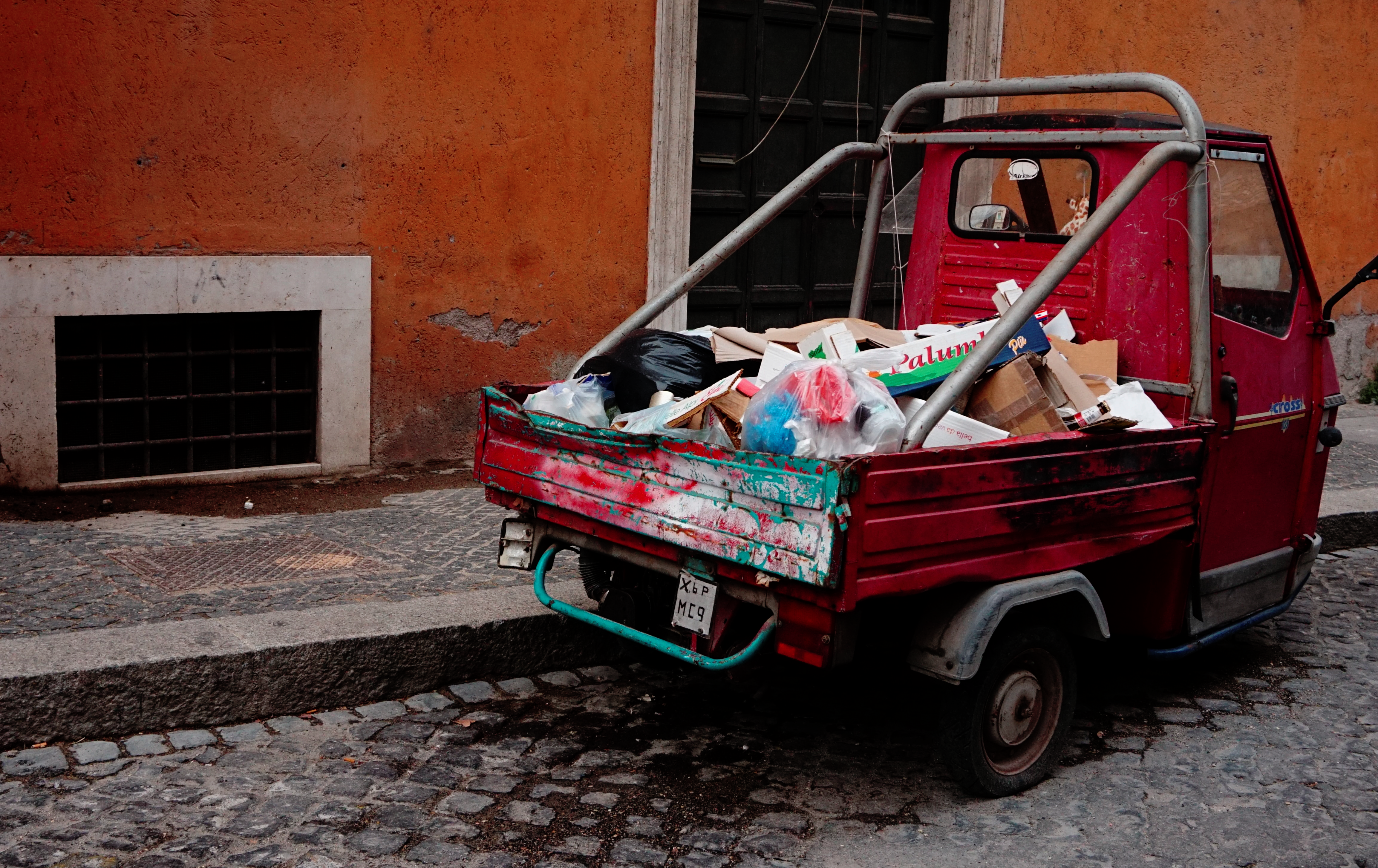
Film simulations from scratch using Python

April 27, 2021April 28, 2021 Kevin8 Comments

Disclaimer: The post is more about understanding LUTs and HaldCLUTs and writing methods from scratch to apply these LUTs to an image rather than coming up with CLUTs themselves from scratch.

Outline

What are film simulations?
CLUTs primer
Simple hand-crafted CLUTs
The identity CLUT
HaldCLUTs
Applying a HaldCLUT
Notes and further reading

There is also an accompanying notebook, in case you want to play around with the CLUTs.

What are film simulations?

Apparently, back in the day, people shot pictures with analog cameras that used film. If you wanted a different “look” to your pictures, you would load a different film stock that gave you the desired look. This is akin to current-day Instagram filters, though more laborious. Some digital camera makers, like Fujifilm, started out as makers of photographic films (and they still make them), and transitioned into making digital cameras. Modern mirrorless cameras from Fujifilm have film simulation presets that digitally mimic the style of a particular film stock. If you are curious, John Peltier has written a good piece on Fujifilm’s film simulations. I was intrigued by how these simulations were achieved and this is a modest attempt at untangling them.

CLUTs primer

A CLUT, or a Color Look Up Table, is the primary way to define a style or film simulation. For each possible RGB color, a CLUT tells you which color to map it to. For example, a CLUT might specify that all green pixels in an image should be yellow:

# map green to yellow
(0, 255, 0) -> (255, 255, 0)

The actual format in which this information is represented can vary. A CLUT can be a .cube file, a HaldCLUT png, or even a pickled numpy array as long as whatever image editing software you use can read it.

In an 8-bit image, each channel (i.e red, green or blue) can take values from 0 to 255. Our CLUT should theoretically have a mapping for every possible color – that’s 256 x 256 x 256 colors. In practice however, CLUTs are way smaller. For example an 8-bit CLUT would divide each channel into ranges of 32 (i.e 256 divided by 8). Since we have 3 channels (red, green and blue), our CLUT can be imagined as a three dimensional cube:

A standard 3D CLUT. Image Credits

To apply a CLUT to the image, each color in the image is assigned to one of the cells in the CLUT cube, and the color of the pixel in the original image is changed to whatever RGB color is in its assigned cell in the CLUT cube. Hence the color (12, 0, 0) would belong to the second cell along the red axis in the top left corner of the cube. This also means that all the shades of red between (8, 0, 0) and (15, 0, 0) will be mapped to the same RGB color. Though that sounds terrible, an 8-bit CLUT usually produces images that are fine to our eyes. Of course we can increase the “quality” of the resulting image by using a more precise (eg: 12-bit) CLUT.

Simple hand-crafted CLUTs

Before we craft CLUTs and start applying them to images, we need a test image. For the sake of simplicity, we conjure up a little red square:

from PIL import Image
img = Image.new('RGB', (60, 60), color='red')
img.show()

We will now create a simple CLUT that would map red pixels to green pixels and apply it to our little red square. We know that our CLUT should be a cube, and each “cell” in the cube should map to a color. If we create a 2-bit CLUT, it will have the shape (2, 2, 2, 3). Remember that our CLUT is a cube with each side of “length” 2, and that each “cell” in the cube should hold an RGB color – hence the 3 in the last dimension.

import numpy as np
clut = np.zeros((2, 2, 2, 3))
transformed_img = apply_3d_clut(clut, img, clut_size=2)
transformed_img.show()

We haven’t yet implemented the “apply_3d_clut()” method. This method will have to look at every pixel in the image and figure out the corresponding mapped pixel from the CLUT. The logic is roughly as follows:

For each pixel in the image:
1. get the (r, g, b) values for the pixel
2. Assign the (r, g, b) values to a “cell” in our CLUT
3. Replace the pixel in the original with the color in the assigned CLUT “cell”

We should be careful with step 2 above – since we have a 2-bit CLUT, we want color values up to 127 to be mapped to the first cell and we want values 127 and above to be mapped to the second cell.

from tqdm import tqdm
def apply_3d_clut(clut, img, clut_size=2):
    """
        clut must have the shape (size, size, size, num_channels)
    """
    num_rows, num_cols = img.size
    filtered_img = np.copy(np.asarray(img))
    scale = (clut_size - 1) / 255
    img = np.asarray(img)
    for row in tqdm(range(num_rows)):
        for col in range(num_cols):
            r, g, b = img[col, row]
            # (clut_r, clut_g, clut_b) together represents a "cell" in the CLUT
            # Notice that we rely on round() to map the values to "cells" in the CLUT
            clut_r, clut_g, clut_b = round(r * scale), round(g * scale), round(b * scale)
            # copy over the color in the CLUT to the new image
            filtered_img[col, row] = clut[clut_r, clut_g, clut_b]
    filtered_img = Image.fromarray(filtered_img.astype('uint8'), 'RGB')
    
    return filtered_img

Once you implement the above method and apply the CLUT to our image, you will be treated with a very underwhelming little black box:

Our CLUT was all zeros, and unsurprisingly, the red pixels in our little red square was mapped to black when the CLUT was applied. Let us now manipulate the CLUT to map red to green:

clut[1, 0, 0] = np.array([0, 255, 0])
transformed_img = apply_3d_clut(clut, img, clut_size=2)
transformed_img.show()

Fantastic, that worked! Time to apply our CLUT to a real image:

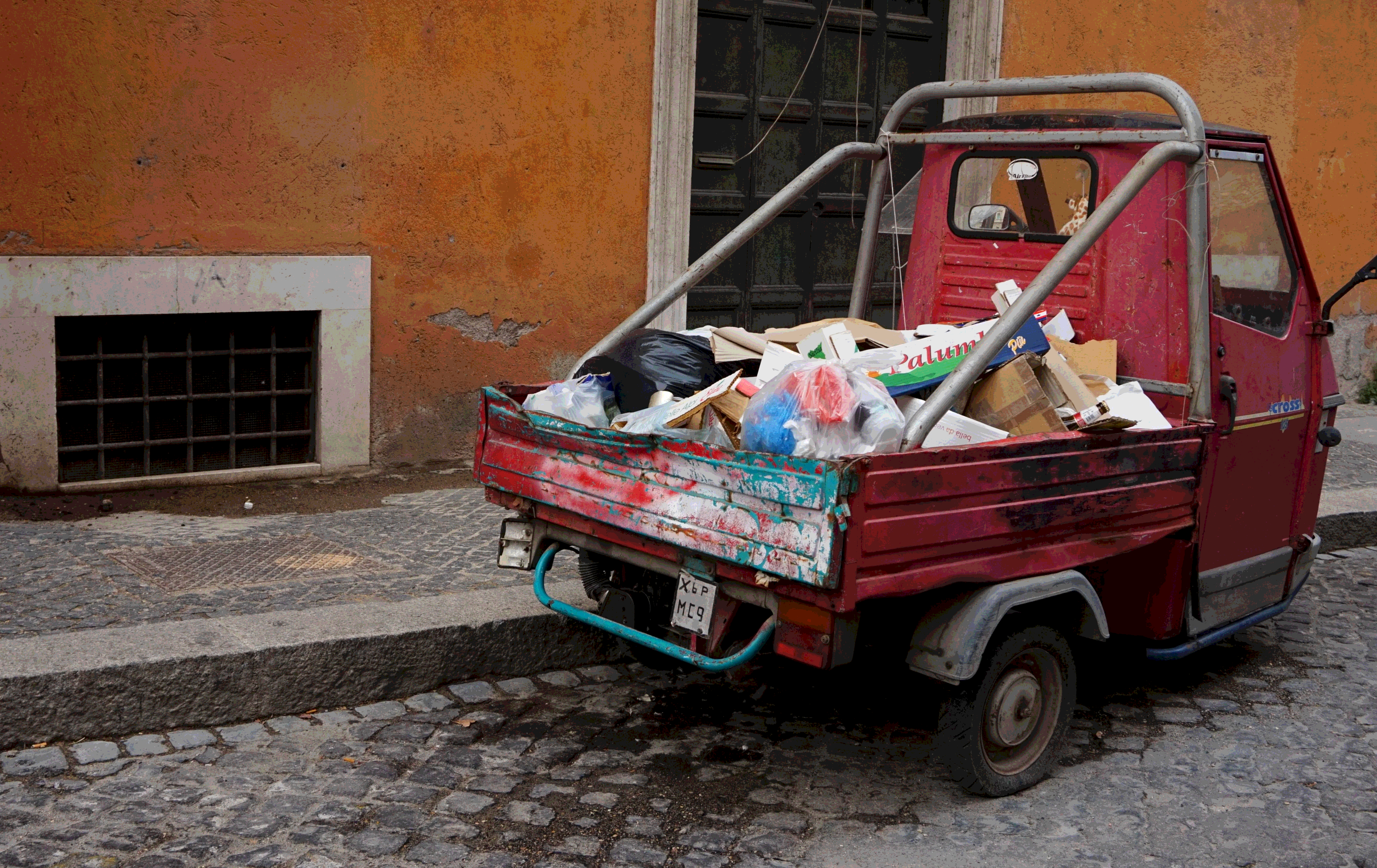
This unassuming Ape truck from Rome filled with garbage is going to be our guinea pig. Our “apply_3d_clut()” method loops over the image pixel by pixel and is extremely slow – we’ll fix that soon enough.

import urllib.request
truck = Image.open(urllib.request.urlopen("https://i.imgur.com/ahpSmLP.jpg"))
green_truck = apply_3d_clut(clut, truck, clut_size=2)
green_truck.show()

That’s a bit too green. We can see that the reds in the original image did get replaced by green pixels, but since we initialized our CLUT to all zeroes, all the other colors in the image was replaced with black pixels. We need a CLUT that would map all the reds to greens while leaving all the other colors alone.

Before we do that, let us vectorize our “apply_3d_lut()” method to make it much faster:

def fast_apply_3d_clut(clut, clut_size, img):
    """
        clut must have the shape (size, size, size, num_channels)
    """
    num_rows, num_cols = img.size
    filtered_img = np.copy(np.asarray(img))
    scale = (clut_size - 1) / 255
    img = np.asarray(img)
    clut_r = np.rint(img[:, :, 0] * scale).astype(int)
    clut_g = np.rint(img[:, :, 1] * scale).astype(int)
    clut_b = np.rint(img[:, :, 2] * scale).astype(int)
    filtered_img = clut[clut_r, clut_g, clut_b]
    filtered_img = Image.fromarray(filtered_img.astype('uint8'), 'RGB')
    return filtered_img

The identity CLUT

An identity CLUT, when applied, produces an image identical to the source image. In other words, the identity CLUT maps each color in the source image to the same color. The identity CLUT is a perfect base for us to build upon – we can change parts of the identity CLUT to manipulate certain colors while other colors in the image are left unchanged.

def create_identity(size):
    clut = np.zeros((size, size, size, 3))
    scale = 255 / (size - 1)
    for b in range(size):
        for g in range(size):
            for r in range(size):
                clut[r, g, b, 0] = r * scale
                clut[r, g, b, 1] = g * scale
                clut[r, g, b, 2] = b * scale
    return clut

Let us generate a 2-bit identity CLUT and see how applying it affects our image

two_bit_identity_clut = create_identity(2)
identity_truck = fast_apply_3d_clut(two_bit_identity_clut, 2, truck)
identity_truck = Image.fromarray(identity_truck.astype('uint8'), 'RGB')
identity_truck.show()

That’s in the same ballpark as the original image, but clearly there’s a lot wrong there. The problem is our 2-bit CLUT – we had a palette of only 8 colors (2 * 2 * 2) to choose from. Let us try again, but this time with a 12-bit CLUT:

twelve_bit_identity_clut = create_identity(12)
identity_truck = fast_apply_3d_clut(twelve_bit_identity_clut, 12, truck)
identity_truck = Image.fromarray(identity_truck.astype('uint8'), 'RGB')
identity_truck.show()

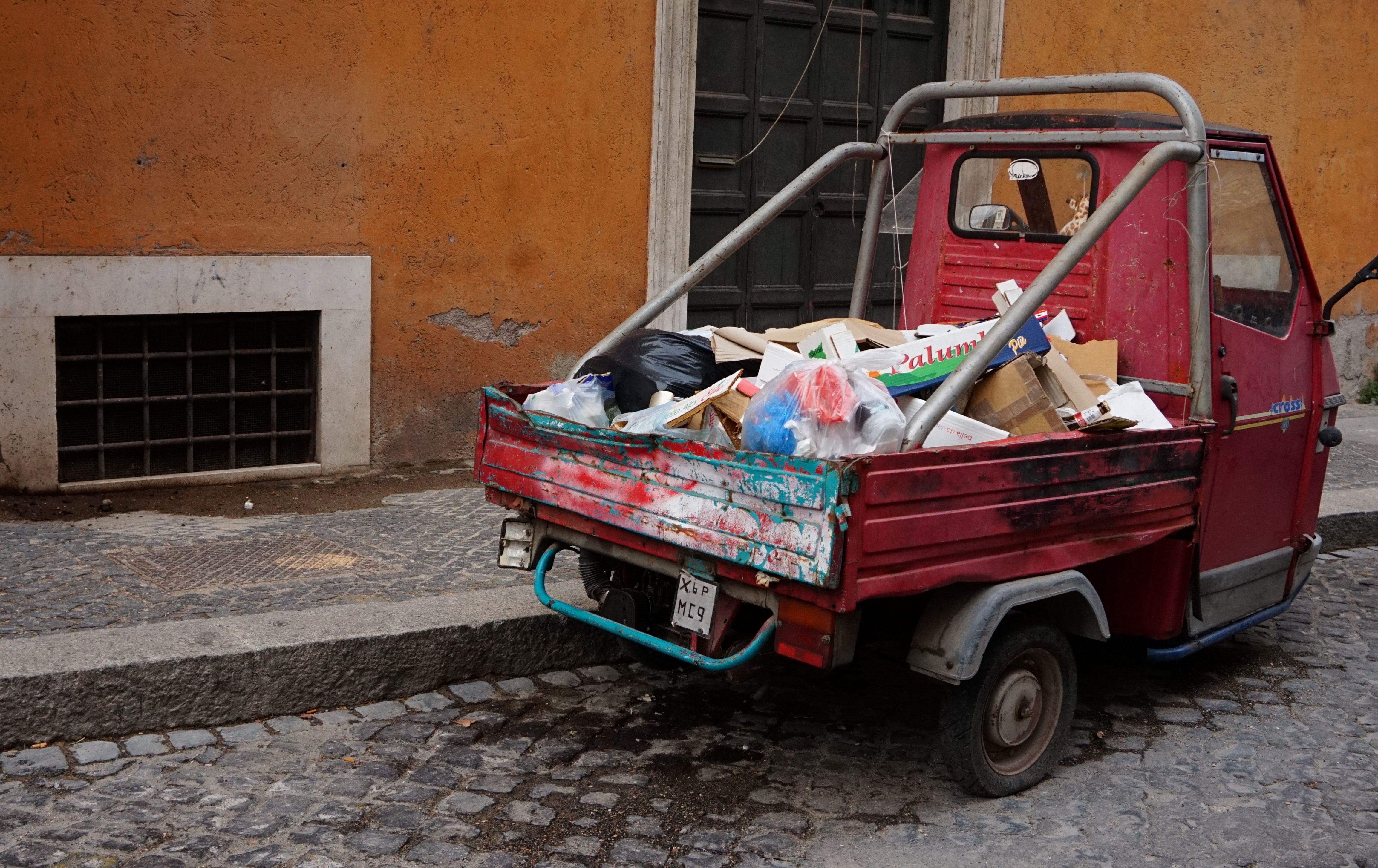
Left – the original image, right – the image after applying the 12-bit identity CLUT

That’s much better. In fact, I can see no discernible differences between the images. Wunderbar!

Let us try mapping the reds to the greens again. Our goal is to map all pixels that are sufficiently red to green. What’s “sufficiently red”? For our purposes, all pixels that end up being mapped to the reddish corner of the CLUT cube deserve to be green.

green_clut = create_identity(12)
green_clut[5:, :4, :4] = np.array([0, 255, 0])
green_truck = fast_apply_3d_clut(green_clut, 12, truck)
green_truck.show()

That’s comically bad. Of course, we got what we asked for – some reddish parts of the image did get mapped to a bright ugly green. Let us restore our faith in CLUTs by attempting a slightly less drastic and potentially pleasing effect – make all pixels slightly more green:

green_clut = create_identity(12)
green_clut[:, :, :, 1] += 20
green_truck = fast_apply_3d_clut(green_clut, 12, truck)
green_truck.show()

Left – the original image, Right – the image with all pixels shifted more to green

Slightly less catastrophic. But we didn’t need CLUTs for this – we could have simply looped through all the pixels and manually added a constant value to the green channel. Theoretically, we can get more pleasing effects by fancier manipulation of the CLUT – instead of adding a constant value, maybe add a higher value to the reds and a lower value to the whites? You can probably see where this is going – coming up with good CLUTs (at least programmatically) is not trivial.

What do we do now? Let’s get us some professionally created CLUTs.

HaldCLUTs

We are going to apply the “Fuji Velvia 50” CLUT that is bundled with RawTherapee to our truck image. These CLUTs are distributed as HaldCLUT png files, and we will spend a few minutes understanding the format before writing a method to apply a HaldCLUT to the truck. But why HaldCLUTs?

HaldCLUTs are high-fidelity. Our 12-bit identity CLUT was good enough to reproduce the image. Each HaldCLUT bundled with RawTherapee is equivalent to a 144-bit 3d CLUT. Yes, that’s effectively CLUT of shape (144, 144, 144, 3).
However, the real benefit of using HaldCLUTs is the file size. Adobe’s .cube CLUT format is essentially a plain text file with RGB values. Since each character in the text file takes up a byte, a 144-bit CLUT in .cube takes up around 32MB on disk. The equivalent HaldCLUT png image file is around a megabyte. But png images are two-dimensional. How can we encode three-dimensional data using a two-dimensional image? We’ll see.

Let’s look at an identity HaldCLUT:

The identity HaldCLUT, generated using `convert hald:12 -depth 8 -colorspace sRGB hald_12.png`

Pretty pretty colors. You’d have noticed that the image seems to have been divided into little cells. Let’s zoom in on the cell on the top-left corner:

We notice a few things – the pixel on the top-left is definitely black – so it represents the first “bucket” or “cell” in a 3D clut and pure blacks (i.e rgb(0, 0, 0)) are going to be mapped to the color present in this bucket . Of course the pixel at (0, 0, 0) in the above image is black because we are dealing with an identity CLUT here – a different CLUT could have mapped the index (0, 0, 0) to gray. The confusing part here is to figure out how to index into the HaldCLUT – let’s say we have a bright red pixel with the value (200, 0, 0) in our source image. If we were dealing with a normal 144-bit 3D CLUT, we would know that a red value of 200 will belong to the index 200 * 144 / 255 = 133 (approximately), and we would replace the color of this pixel with whatever was at CLUT[113][0][0]. But we are not dealing with a 3D CLUT here – we are dealing with a 2-D image, while we have to index into this image as if it was a 3D CLUT.

The entire identity HaldCLUT image in our example has the shape (1728, 1728), and each of those little cells that you see has the shape (12, 144), and there are 144 such cells in a single column of the image (i.e vertically). The HaldCLUT, as you can see, has 12 columns. Hence we have 1728 cells in the entire HaldCLUT, each cell having the shape (12, 144). This is how we index into a HaldCLUT file:

(if the description doesn’t make much sense, it is followed by a code snippet that’s hopefully clearer)

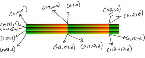
Within each cell, the red index always changes from left to right. In our top-left cell, it changes from 0 to 143. This is the case in each row within each cell – the red index is always 0 in the first column of a cell, and 1 in the second column and so on. Since each cell has 12 rows, in each of these rows the red index changes from 0 to 143.
The green index is constant in each row within a cell, and increments by 1 across cells horizontally, and wraps around. So the pixel at position (143, 0) in the HaldCLUT image represents the index (143, 0, 0), while the pixel at position (144, 0) represents the index (0, 1, 0) and so on. The pixel at position (1, 0) would represent the index (0, 12, 0).
The blue channel is constant everywhere within a cell, and increments by 1 across cells vertically. So the pixel at position (11, 0) will represent the index (0, 131, 0) while the pixel at (12, 0) will represent the index (0, 0, 1). Notice how both the red-index and green-index was reset to 0 when moved down the HaldCLUT image by an entire cell.

The top-left corner extracted from the full identity HaldCLUT. Only the first 3 rows and two columns are shown here (the third column is clipped). Note that the annotations represent the index into the 3d CLUT that pixel represents if the HaldCLUT was instead a normal 3D CLUT. Each cell has the shape `(12, 144)`. When there are two lines in the diagram seemingly coming out from the same pixel, I am trying to show how the represented index changes between adjacent pixels at a cell boundary.

Inspecting the identity HaldCLUT in python reveals the same info:

identity = Image.open("identity.png")
identity = np.asarray(identity)
print("identity HaldCLUT has size: {}".format(identity.shape))
size = round(math.pow(identity.shape[0], 1/3))
print("The CLUT size is {}".format(size))
# The CLUT size is 12
print("clut[0,0] is {}".format(identity[0, 0]))
# clut[0,0] is [0 0 0]
print("clut[0, 100] is {}".format(identity[0, 100]))
# clut[0, 100] is [179   0   0]
print("clut[0, 143] is {}".format(identity[0, 143]))
# We've reached the end of the first row in the first cell
# clut[0, 143] is [255   0   0]
print("clut[0, 144] is {}".format(identity[0, 144]))
# The red channel resets, the green channel increments by 1
# clut[0, 144] is [0 1 0]
print("clut[0, 248] is {}".format(identity[0, 248]))
# clut[0, 248] is [186   1   0]
# Notice how the value in the green channel did not increase. This is normal - we have 256 possible values and only 144 "slots" to keep them. The identity CLUT occasionally skips a 
print("clut[0, 432] is {}".format(identity[0, 432]))
# clut[0, 432] is [0 5 0]
# ^ The red got reset, the CLUT skipped more values in the green channel and now maps to 5. This is the peculiarity of this CLUT. A different HaldCLUT (not the identity one) might have had a different value for this green channel step.
print("clut[0, 1727] is {}".format(identity[0, 1727]))
# clut[0, 1727] is [255  19   0]
# This is the last pixel in the first row of the entire image
print("clut[1, 0] is {}".format(identity[1, 0]))
# clut[1, 0] is [ 0 21  0]
# Notice how the value in the green channel "wrapped around" from the previous row
print("clut[1, 144] is {}".format(identity[1, 144]))
# Exercise for the reader: see if you can guess the output correctly 🙂
print("clut[12 0] is {}".format(identity[12, 0]))
print("clut[12 143] is {}".format(identity[12, 143]))
print("clut[12 144] is {}".format(identity[12, 144]))

Applying a HaldCLUT

Now that we’ve understood how a 3D CLUT is sorta encoded in a HaldCLUT png, let’s go ahead and write a method to apply a HaldCLUT to an image:

import math 
def apply_hald_clut(hald_img, img):
    hald_w, hald_h = hald_img.size
    clut_size = int(round(math.pow(hald_w, 1/3)))
    # We square the clut_size because a 12-bit HaldCLUT has the same amount of information as a 144-bit 3D CLUT
    scale = (clut_size * clut_size - 1) / 255
    # Convert the PIL image to numpy array
    img = np.asarray(img)
    # We are reshaping to (144 * 144 * 144, 3) - it helps with indexing
    hald_img = np.asarray(hald_img).reshape(clut_size ** 6, 3)
    # Figure out the 3D CLUT indexes corresponding to the pixels in our image
    clut_r = np.rint(img[:, :, 0] * scale).astype(int)
    clut_g = np.rint(img[:, :, 1] * scale).astype(int)
    clut_b = np.rint(img[:, :, 2] * scale).astype(int)
    filtered_image = np.zeros((img.shape))
    # Convert the 3D CLUT indexes into indexes for our HaldCLUT numpy array and copy over the colors to the new image
    filtered_image[:, :] = hald_img[clut_r + clut_size ** 2 * clut_g + clut_size ** 4 * clut_b]
    filtered_image = Image.fromarray(filtered_image.astype('uint8'), 'RGB')
    return filtered_image

Let’s test our method by applying the identity HaldCLUT to our truck – we should get a visually unchanged image back:

identity_hald_clut = Image.open(urllib.request.urlopen("https://i.imgur.com/qg6Is0w.png"))
identity_truck = apply_hald_clut(identity_hald_clut, truck)
identity_truck.show()

Let us finally apply the “Fuji Velvia 50” CLUT to our truck:

velvia_hald_clut = Image.open(urllib.request.urlopen("https://i.imgur.com/31UrdAg.png"))
velvia_truck = apply_hald_clut(velvia_hald_clut, truck)
velvia_truck

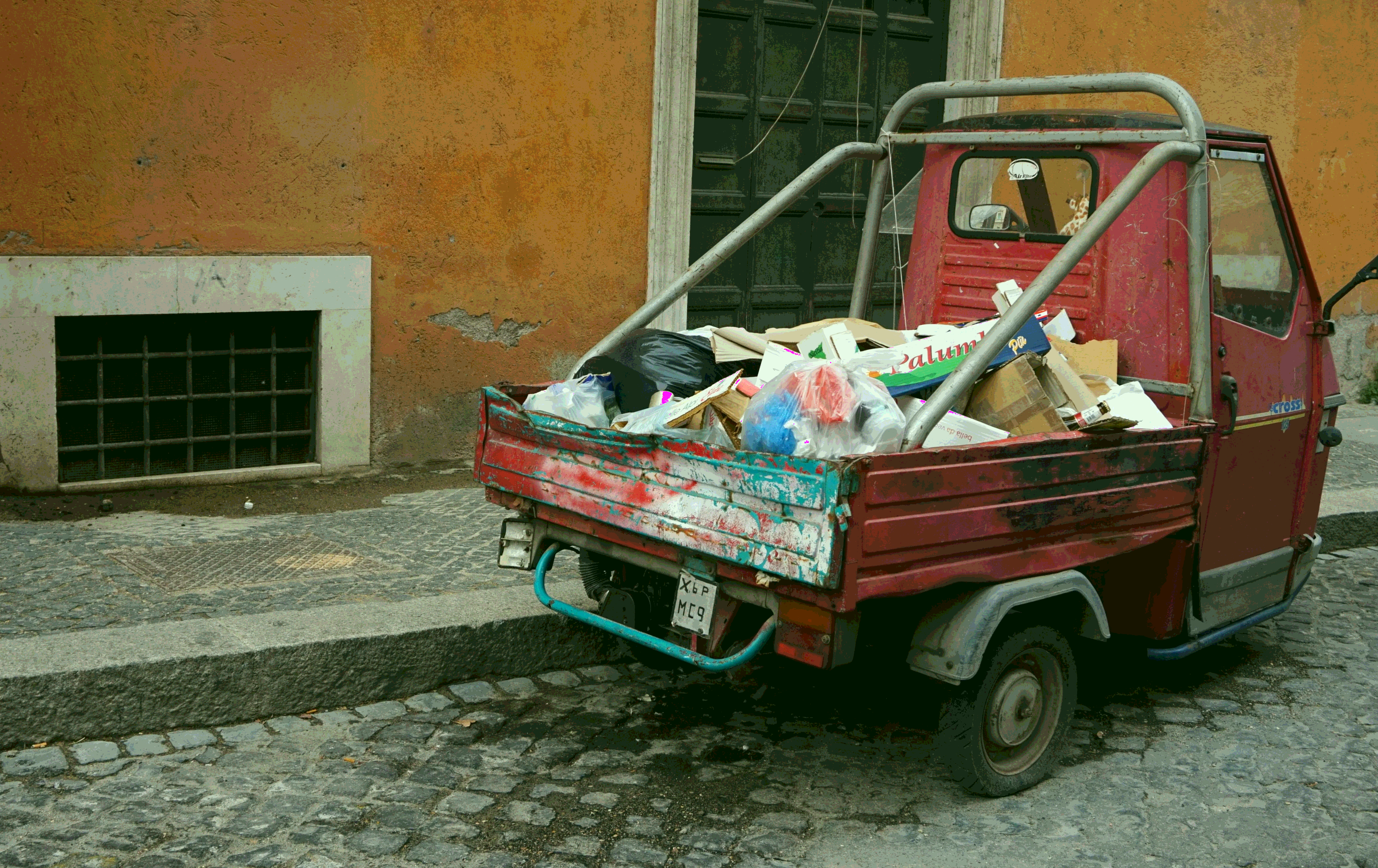
Left – the original image, Right – image after apply the “Fuji Velvia 50” HaldCLUT

That worked! You can download more HaldCLUTs from the RawTherapee page. The monochrome (i.e black and white) HaldCLUTs won’t work straight-away because our apply_hald_clut() method expects a hald image with 3 channels (ie reg, green and blue), while the monochrome HaldCLUT images have only 1 channel (the grey value). It won’t be difficult at all to change our method to support monochrome HaldCLUTs – I leave that as an exercise to the reader 😉

Notes and further reading

Remember how we saw that a 2-bit identity CLUT gave us poor results while a 12-bit one almost reproduced our image? That is not necessarily true. Image editing softwares can interpolate between the missing values. For example, this is how PIL apply a 3d CLUT with linear interpolation.

The “Fuji Velvia 50” HaldCLUT that we use is an approximation of Fujifilm’s proprietary velvia film simulation (probably) by Pat Davis

If you want to create your own HaldCLUT, the easiest way would be to open up the identity HaldCLUT png file in an image editing software (e.t.c RawTherapee, Darktable, Adobe Lightroom) and apply global edits to it. For example, if you change the saturation and contrast values to the HaldCLUT png using the image editor, and apply this modified HaldCLUT png (using our python script, or a different image editor – doesn’t matter how) to a different image, the resulting image would have more contrast and saturation. Neat right?

Programming: doing it more vs doing it better

April 8, 2019April 8, 2019 Kevin10 Comments

A few years ago, very early into my programming career, I came across a story:

The ceramics teacher announced on opening day that he was dividing the class into two groups. All those on the left side of the studio, he said, would be graded solely on the quantity of work they produced, all those on the right solely on its quality. His procedure was simple: on the final day of class he would bring in his bathroom scales and weigh the work of the “quantity” group: fifty pound of pots rated an “A”, forty pounds a “B”, and so on. Those being graded on “quality”, however, needed to produce only one pot – albeit a perfect one – to get an “A”.
Well, came grading time and a curious fact emerged: the works of highest quality were all produced by the group being graded for quantity. It seems that while the “quantity” group was busily churning out piles of work – and learning from their mistakes – the “quality” group had sat theorizing about perfection, and in the end had little more to show for their efforts than grandiose theories and a pile of dead clay.
Jeff Atwood’s “Quantity Always Trumps Quality” post, though he himself took the story from somewhere else.

This little story has had a tremendous impact on how I approach software engineering as a craft. I was (and still am) convinced that the best way to get better at software engineering is to write more software. I was careful enough to not take the story too seriously – I have always strived to write readable, maintainable code without bugs. However, deep inside my mind was this idea that one day I would be able to write beautiful code without thinking. It would be as effortless to me as breathing. “Refactoring code” would be something left to the apprentice, not something that I, the master who has churned out enough ceramic pots, would be bothered with. I just have to keep making ceramic pots until I get there.

Three years later, I am still very much the apprentice. Rather than programming effortlessly, I have learned to program more deliberately. I have learned (the hard way) to review my code more thoroughly and to refactor it now rather than later. I get pangs of guilt and disappointment every time my pull request has to go through another round of review. I am frustrated when I deliver a feature two days late. As an engineer I want to, above everything else, churn out (the right) features as fast as possible.

Today, I came across an essay that would let me resign from my perpetual struggle to “get faster” at engineering:

I used to have students who bragged to me about how fast they wrote their papers. I would tell them that the great German novelist Thomas Mann said that a writer is someone for whom writing is more difficult than it is for other people. The best writers write much more slowly than everyone else, and the better they are, the slower they write. James Joyce wrote Ulysses, the greatest novel of the 20th century, at the rate of about a hundred words a day
William Deresiewicz, Solitude and Leadership

I can strongly relate to this – I would often read and re-read something that I wrote and then I would go back and change it, only to repeat the process again. Though comparing my modest penmanship (keymanship?!) to “the best writers” is outright sacrilegious, even I have in the past noticed that the slower I write, the better I write.

The equivalent in software engineering terms would be to (nothing you did not know before, except for maybe the last point):

Put more thought into the design of your systems
Refactor liberally and lavishly
Test thoroughly
Take your sweet time

As I said, nothing you did not know before. Also, this is almost impossible to pull off when you have realistic business objectives to meet.

But James Joyce probably did not write Ulysses with a publisher breathing down his neck saying “We need to ship this before Christmas!”.

So the secret sauce that makes good code great and the average Joe the next 10x programmer might be this – diligence exercised over a long time.

How does this affect me? Disillusionment. Writing more software does not automatically make you a better programmer. You need the secret sauce, whatever that might be.

Announcing matchertools 0.1.0

March 7, 2019March 7, 2019 KevinLeave a comment

Matchertools is my “hello world” project in rust, and I have been chipping away at it slowly and erratically for the past couple of months. You can now find my humble crate here. The crate exposes an API that implements the Gale-Shapley algorithm for the stable marriage problem. Read the wiki. No really, read the linked Wikipedia page. Lloyd Shapley and Alvin Roth won a Nobel prize for this in 2012. Spoiler alert – unlike what the name indicates, the algorithm has little to do with marriages.

This project is so nascent that it is easier for me to list what it does not have:

No documentation
No examples
Shaky integration tests
No code style whatsoever. I haven’t subjected the repo to rustfmt yet (gasp!)
Duct-tape code.
Not nearly enough code comments.

Web design for programmers : A 10 minutes crash course

February 3, 2015 Kevin2 Comments

I’m not a designer, and I’d rather not be one. However, there are times when programmers who don’t like to design (or draw, for that matter) are forced into that tedious act. I was responsible for designing the front end of a product at a company I interned at for the last 2 months.

Needless to say, html + css was terrifying for me. There were days where I spent entire mornings trying to align the bloody divs. Also, my choice of colors and “ui elements” were not at all pleasing. I had to pull this together somehow. I scoured the web for some intro to design. So here’s what 2 months of front-end taught me :

1. For the love of God, use bootstrap. No matter how promising the control and flexibility of pure css looks, use bootstrap and save the headache – at least when you start out.

2. Use a pen and paper to sketch your design. If you don’t like pens or papers, use a wireframing tool such as wireframe.cc. I spent some considerable time building wireframes, and then threw them away when I changed the design. Lesson learned – use pen and paper. Wireframes are useful when you want a more detailed/accurate layout of your web app.

3. Chances are that you are terrible at choosing colors. Use a tool like paletton to find the right colors, and the right combination of colors.

4. Use good fonts. Microsoft’s Segoe UI is now my favourite font. Segoe UI wasn’t featured in even a single article that discussed the “best free web fonts”. Experiment.

5. Don’t use too many colors, and don’t use too many fonts. Try to keep it simple whenever possible.

6. The official bootstrap docs does not contain references of some really useful bootstrap components like “panel” and “panel-default”. So be sure to double check before you decide that bootstrap doesn’t have it already.

7. You can’t come up with a “mind blowing, innovative, revolutionary design” over night. You might, but chances are that you won’t. Always try to build upon designs (please don’t use templates) that already exist. Here are some useful links for you to ‘build-upon’ :

Another programmers intro to design
Wireframing for beginners
People have been praising and praising mailchimp’s new UI – article.
https://goodui.org – If you are trying to sell something
Quora design notes

8. Don’t be afraid to rewrite the HTML. I had to design a signup form and my first implementation sucked. The HTML was a mess and I couldn’t even think of modifying it. So I just wrote that page again, from scratch. Not only did I come up with a wonderful new design and styling (hint: tiles and css shadow on hover), the HTML was much much more readable. Break and build, break and build.

Good luck.

Cohen’s clipping algorithms

October 27, 2014 Kevin1 Comment

Okay this was homework. I searched for a really long time for a javascript implementation of cohen’s clipping algorithms and could find none. Professor said write it in c but its hard to program mouse clicks in c. With javascript, all it takes is a browser.

1. Cohen-sutherland line clipping algorithm in javascript

2. Sutherland-Hodgman polygon clipping algorithm in javascript.

I believe the code is pretty readable – I had commented lavishly. Save them as html files, open in a browser, and keep clicking left mouse button.

And yes, the implementation is not perfect. I basically drew over the edges in white to “erase” it and that is why you see a very thin line outside the rectangle in the image.

Sound frequencies with aubio

October 21, 2014 KevinLeave a comment

Small python script I wrote so that you can yell at the console and see the frequency on the screen. The results can be slightly wrong (incorrect spikes in frequency occasionally) but it was great yelling at the computer with my hostel mates to see who’s got the highest ‘range’ 😀

Link to the github gist.

The code is too small to give an explanation. However, you need to set up a few libraries before running the gist (instructions for linux) :

1. aubio – A fantastic library for analysing audio. Packages libaubio and python-aubio are available in the ubuntu/mint repositories. However, I ran into problems (repos have older versions I guess) and was able to fix them only after compiling the source. So head over to this repo, download the source code, and compile.

To compile aubio, head over to the source directory and type:

./waf configure

That will spew out a list of packages you will need at the end. Make sure you install the dev versions of each package. For example, for sndfile, do

sudo apt-get install libsndfile1-dev

Similarly install all the packages that you would need to use with aubio. I did not have a clue as to what I will need so I installed them all.

Now do ./waf build
and then sudo ./waf install

That should install aubio on your linux system. Time to install the python wrappers. ‘cd’ to /python directory in the aubio source.

python setup.py build to build the files and after building,
sudo python setup.py install to install the python wrappers for aubio

2. The snippet depends on pysoundcard, which is not available in the repos. Head over here to download the source. Build and install this python package the same way you did the aubio python wrappers

Download (or type) the gist and run it! Happy yelling!

GSoC : Final report

August 21, 2014 KevinLeave a comment

Putting together a quick report of how I spent my last 3 months on improving varnam, an awesome transliteration project. My task was to implement a stemmer to improve the learning in varnam.
A stemmer is an algorithm that, upon giving a word as the input, gives the base word as the output.

For example, giving മരത്തിലൂടെ as the input would give you മരത്തിൽ and മരം as outputs. മരം is the final output of the stemmer and മരത്തിൽ is an intermmediate output of the stemmer. The algorithm is described here. The stemmer is similar to SILPA stemmer created by Santhosh Thottingal except that my version makes use of an exceptions table and produces meaningful intermmediate words.

A screencast that explains my work is posted above. Make sure you watch it in 720p to clearly see the words being typed.

As far as statistics go, see this thread to know how much the learning has improved. This is not the final result, as the number of words learned is of no consequence if the stemmer does not improve transliteration accuracy. Transliteration accuracy tests before and after the tests are yet to be done thoroughly. Judging by the number of new words in the word corpus alone, varnam saw an improvement of 63% in learning when tested with 408 words.See the above thread for the exact results and the word corpus used.

GSoC : Memory heap corruption and code rewrite

July 31, 2014 KevinLeave a comment

This week I’ve been busy rewriting the stemmer and debugging some memory heap corruption. My first implmentation of the stemmer used to crash ibus whenever certain words, like “ദൂരെയാണ്” and “വിദൂരമായ” were typed. I could not locate the problem, and the only error message I got was “free() – invalid next size” when ibus crashed. Some searching revealed that it might be due to a memory heap corruption. I used valgrind memcheck to debug the memory corruption. It was difficult to make sense of valgrind’s output, and that eventually lead me to ask a question at stackoverflow. However, before all this, I was convinced that I made some serious mistake somewhere along the development path and decided to sit down and rewrite the whole project. I thought that I made a mistake by not testing with ibus early on. I discovered what I was doing wrong to merit the memory corruption soon after (even before the guy came in and gave his answer at stackoverflow.com). However, I realised that a rewrite would do the project much good. To start with, I could then run valgrind as I went with the rewrite to make sure that I plugged all the possible memory leaks. Also, I was able to look into some unnecesary function calls among other things. In short, I cleaned the code and is ready for a code review.

Here’s a changelog:

1. Tried implementing the “improvement scheme”, as I had suggested in this thread. The results were far worse than expected. 60% of the words after suffix appending were not meaningful. Any further attempts along this path would require much more careful planning and reasearch of the malayalam language.

2. Located and avoided [did not stonewall it] an annoying memory corruption. Filed it under issue 51.

3. Removed the level hierarchy. All stemrules are now grouped into one. Splitting the stemrules into 3 levels serve no real purpose, and complicates stemming by needing to check each level seperately. Also, removal of the level system has improved the code readability a lot.

4. Replaced some function calls with inline expansions. Made all the functions more defensive and freed memory wherever valgrind reported memory leaks.

5. Libvarnam ibus requires a clean build every time libvarnam.so changes. It seems that libvarnam-ibus has its own version of libvarnam or something. Should look into this. Ibus not reflecting the changes I made to libvarnam was a real headache – no amount of debugging could solve the issue. Tried recompiling libvarnam-ibus and things started to work.

6. Eliminated recursive calls to varnam_learn(). In the first implementation, varnam_learn() would call varnam_stem() which calls varnam_learn_internal(). This was bad design. Now varnam_stem() returns a varray to varnam_learn(), and varnam_learn() iterates over this varray to learn all the stemmed words.

These changes are not final. Some of it, like doing away with the level system, was done without consulting my mentor and would be reintroduced if he thinks that removing it was a bad decision. You can see all my changes here and make suggestions.

To do :

1. More tests
2. Make sure stemmer works well with other languages
3. Enable varnam to stem from the command line interface

GSoC : Code review 1, almost.

July 20, 2014 KevinLeave a comment

Before more thorough testing of the stemming algorithm and its effect on varnam’s learning, my mentor and I decided that it would be a good idea to do some code review. So this week I fixed some problems with the stemming, tested how the stemming works with ibus input method, checked if learning is improving at all, and wrote some unit tests.

Stemming with IBus works, though with some bugs. Let us consider a case that works. The learnings database is now empty and we are starting with the blank state. Varnam does not know anything other than the symbols specified in the scheme file.
The below video demonstrates varnam learning a word with Ibus as the input method. The next time the user starts to type the same word, you can see that its stemmed forms are available in the suggestions.

Right now the only cause of concern with the suggestions is that incomplete words are suggested first, and the user has to go through the suggestions list to find the intended word. Also each time varnam learns a stemmed word, all its prefixes are learned as well. This will eventually lead to the incomplete prefixes coming up first on the suggestions list and the user will have to look through the list to find the word she is looking for.

There are some bugs, like some words dissappearing when I choose them from suggestions. The varnam_stem() function is possibly modifying some things that it isn’t supposed to. I’m also getting errors when I’m using free() – invalid next size(fast). Maybe the upcoming code review will expose my mistakes.

Category: programming