I’ve been thinking about binary neural networks lately, and specifically how to do it without computing full precision gradients.
Broadly, there are two camps in binary neural networks. The most prominent (and effective) way to train binary neural networks is to keep the weights in full precision and binarise during forward pass. I’d say BitNet and ReactNet falls under that camp. The problem is of course that you are not taking advantage of the binary weights during the backward pass. Most binary NNs are motivated by the need for fast inference, not training, so full precision backward passes are not generally considered a problem. In fact, keeping latent full-precision weights (i.e non-binary weights) in memory during training is a tried-and-tested technique to train binary neural networks that don’t suck.
But, Shibuya et. al has been doing research on training binary neural networks without keeping a copy of the weights in full-precision in memory. They had an ICLR 2024 submission that unfortunately didn’t get accepted, and then a more recent paper titled Binary Stochastic Flip Optimization for Training Binary Neural Networks. They still use real-valued gradients, but they keep the weights binary throughout the training. The core idea is very intuitive:
Imagine a neural network with binary weights (0 and 1)
The activation function is a sign() function. This is of course not differentiable. So you use a straight-through-estimator (STE) as an approximation. Essentially, you pretend that you were using a hard-tanh as an activation function and compute the gradients as if you were using this tanh activation instead of sign()
The gradient computation proceeds normally – for a weight matrix W_l from layer l, you will have real-valued gradients. Let’s call this gradient matrix G_l
If we were using standard real-valued SGD, the weight would be updated as
Where
is the learning rate, and is usually a small value like 0.001
But you want to keep the weights W_l binary. If you add real-valued gradients to binary W_l, the updated weights will be no longer binary.
The authors get around this problem by simply binarising -G_l. Positive gradient values will be replaced by 1 and negative values will be replaced by a 0
But you can’t just add the binarised gradients to the weight matrix. That would be conceptually equivalent to having a learning rate of 1! That’s too high! And since the gradient matrix is now binary, there’s no concept of a “learning rate”.
Remember, G_l is now a binary matrix, and tells you what the updated weight matrix would look like. Conceptually, if our learning rate (whatever that means – bear with me) was 1, we would just add the gradient matrix to the weight matrix. In our case, instead of adding the gradient matrix to the weights, we would just replace the weight matrix with the gradient matrix. This is the ugly side effect of using binary weights.
Let that sink in. When your gradients are binarised, you can’t “add” the gradient to the weight. The gradient value is going to be either a 1 or a 0. Your weight too is going to be either a 1 or a 0. Your decision is to either match the gradient value or not to match it. For example, if the weight is 0 and the gradient is 1, you have no option but to set the weight to 1 – because that’s what the gradient is telling you to do in order to minimise the loss!
But if we do what the binarised gradient tell us to do, we’ll be flipping our binary weights all the time. In other words, our learning rate is too high! But what does it mean to have a “low” learning rate when the gradient matrix just contains 1s and 0s?
The authors of Binary Stochastic Flip paper suggest that we use a binary mask and do an element-wise multiplication with the gradient matrix. This way, you can select a subset of the gradient matrix to be applied. In other words, instead of setting all the weights according to the gradient matrix, we update only a fraction of the (eg: 10%) of the weights to match the gradient matrix. When the learning rate is “1” (or when it is “maximum”), the mask is a tensor with every element set to 1. To user a lower learning rate, the mask matrix is created in such a way that it will only have a few ones.:
represents element-wise multiplication. Multiplying the existing weight with selects the elements from the original weight that we want to keep. Everything else is zeroed-out. Adding to this sets these zeroed out elements to the value in the gradient matrix
The paper even mentions that setting the Mask randomly works rather well.
In PyTorch, I think it will look something like this:
class HyperMaskOptimizer(Optimizer):
    def __init__(self, params, delta=1e-3):
        """
        Args:
            params: Model parameters (binary weights in {0,1})
            delta: Probability for random mask (δ_t in paper)
        """
        defaults = dict(delta=delta)
        super(HyperMaskOptimizer, self).__init__(params, defaults)
        self.delta = delta

    def step(self, closure=None):
        for group in self.param_groups:
            for param in group['params']:
                grad = param.grad

                current_weights = param.data.clone()  # w_{t-1} in {0,1}
                target_weights = (-grad >= 0).float()  # w*_t in {0,1}

                mask = torch.bernoulli(torch.full_like(grad, self.delta))
                mask_not = 1 - mask  # m̄_t (NOT operation)

                new_weights = (mask_not * current_weights) + (mask * target_weights)

                param.data.copy_(new_weights)
I wasn’t able to reproduce the numbers that the authors reported. Here’s my implementation. My 4-layer perceptron achieved only an unimpressive 33% test accuracy on MNIST after training for 200 epochs. Unfortunately the paper does not mention a reference implementation for me to cross-check with. I’ve reached out to someone whose name matches with that of the first author on LinkedIn. If I’m lucky, they’ll open source their implementation.
Meanwhile, if you can spot bugs in my snippet, please comment on the Github gist (or here) 😀
When I was at Amazon’s LLM pre-training team, our pre-training jobs used to run for weeks. Being impatient as I am, it was frustrating to wait for a whole week to see if the changes we made (mostly to the data) worked. The magic number was 1 trillion tokens, and even a smallish model (eg: 7 billion parameters) will take a few days to reach this point even with the amount of GPUs we had access to.
Now imagine you want to pre-train a model. All you have is access to one GPU, let’s say you want to train it on all of slimpajama and you want to be done with pre-training in a day. That’s roughly 600 billion tokens. Currently, this is a pipe dream. For a model to be trained on 600B tokens a day, your training throughput needs to be 7 million tokens a second. The typical training speeds you see are sub 10k tokens per second per GPU:
And we are talking about 7 million tokens per second. Even if we assume 100% utilisation of the hardware (which is rare), we’ll end up with some pretty small theoretical limits to how large our model can be. Let’s try to work that out.
Target 7 million tokens/sec – how large can our model be?
To process 7 million tokens a second, the model will have to do quite a lot of floating point operations per second:
But there are theoretical upper limits for the number of floating point operations the GPU can do per second.
Let’s assume that FLOPs for backward pass is 2.5x that of the forward pass. This is the assumption made in FlashAttention2 paper and likely holds only for self-attention, but it sounds like a reasonable assumption. Let’s also assume that every parameter in the model results in 2 FLOPs in the forward pass – every parameter in a weight matrix will be involved in one multiplication and one addition as part of matmul. Let’s ignore other layers (eg: softmax, layer norm) for the time being:
If we substitute FloatComputationsPerSecond with 950, which is the theoretical best we can get (on an H100), we’ll have to limit our model to 19.3 million parameters if the training is to proceed at 7 million tokens per second. If we assume a more realistic 40% utilisation of the GPU (350 TFLOPS), we’ll be limited to 7 million parameters for our model.
During inference, we can quantise the model to improve inference speed by multiples while losing only a fraction of the accuracy. Why can’t we do that during training? Better yet, why can’t we go all the way and make all our weights binary? Yes, we will lose model performance, but it is not obvious if model training will be much faster.
But is computation even the bottleneck?
Even if your model fits in a single GPU, large distributed pre-training runs (i.e data-parallel runs) are often bottlenecked by the communication overhead. Each GPU has a copy of your model and computes its gradients. At the end of the backward pass, you must average the gradients across all GPUs. This all_reduce step can absolutely be a bottleneck.
If your model is too big to fit in a single GPU, then you must use model-parallelism to shard the model across multiple GPUs. This introduces yet another network bandwidth-heavy operation (all_gather)
You also have to read data from the disk, and in case of data-parallel runs, probably from a network-mounted drive.
So no, computation is usually not the bottleneck.
But, if your model fits in a single GPU and you are not using data-parallelism, then you have zero communication overhead and training might indeed be limited by compute.
Can’t you just use a lower precision during training?
Yes you can. The newer H100 GPUs introduced fp8 tensor cores and Nvidia’s Transformer Engine reports a 1.46x speedup when training Llama3 8B with fp8. It is harder to achieve stable training with lower precision floats or integers – the first successful fp4 pre-training is very recent.
Has anyone tried using binary weights? Not really. There’s BitNet and the variants. However, they don’t report training throughput numbers. Moreover, I wouldn’t expect training throughput to improve since BitNet maintains latent weights in full precision and the weights are binarised on-the-fly during forward pass. There’s Training Binary Neural Networks in a Binary Weight Space by Shibuya et. al, and that’s the closest work I could find that trains a binary neural network without having to compute latent weights in full precision. However, the authors do not mention how they implemented the binary weights – for all I know the weights were still fp32 but artificially confined to values of +-1. I suspect this is why table 2 in the paper reports analytical memory usage rather than experimental memory usage. It’s a pity that the paper was rejected for ICLR 2024. All the reviewers gave high “soundness” and “contribution” scores and then proceeded to criticise the experiments section. One reviewer mentioned that “the experimental results in Tab.3 seem extremely bad on medium-sized datasets such as CIFAR-10 and Tiny-ImageNet” – but that’s not the point! The results were proof that the method worked, and that should have been sufficient to justify an acceptance. Also, the “extremely bad” error rate 2.5% for the binary network vs 1.46% for the full precision baseline. The circus of academic publishing. But I digress.
Let’s not even talk about memory, apart from just stating that compared to fp16, binary weights will take 16x less memory.
But why would computation be sped up? Imagine taking the dot product of two float vectors of size n. This will require n multiplications and n additions, for a total of 2n floating point operations. Now imagine your vectors were binary and the values were confined to -1 or +1. Instead of doing a dot product, you can now represent your vectors as two integers – also known as a packed integer – and do an xnor + bitcount operation to get the same result as a naive dot product. That’s just 2 operations, compared to 2n operations for a dot product, resulting in theory a speedup by a factor of n. See the figures below
Figure 1: Naive dot product resulting in n multiplications and n additions
The intuition is as follows – when all the elements in the vector are all either -1 or 1, the result of multiplication (when you do a dot product) of two elements is 1 if they are the same (i.e both are 1 or both are -1). If the elements are not the same, the result of multiplication is -1. The dot product is just a sum of these element-wise multiplications. So the final result of dot product can be seen as “the number of 1 results minus the number of -1 results in element-wise multiplication.”.
This is exactly what an XNOR (i.e an exclusive NOR) does – it outputs “1” if both the operands are 1s or 0s. If the elements are not the same (i.e 1 and 0 or 0 and 1), the output of XNOR is 0. GPUs (and CPUs) provide a single operation to count the number of set bits in an integer, called population count. In CUDA, it’s the __popc() function. The XNOR-Net paper popularised this. Thus we can re-write the dot product for binarised vectors a and b as:
If a and b are binary vectors of length 64, they can be represented by a single 64-bit integer each. CUDA provides a __popc() method that is a single operation that returns the number of set bits (i.e 1s) in an integer. Since length of a and b are the same – call it n – and numberOfOnes is given by the __popc() method in CUDA:
dot(a,b) = 2 x __popc(~(a^b)) – n
That is, the dot product of two vectors of length 64 takes 3 operations – a multiplication by 2, the __popc() and the addition with -n. See figure 2 below for an example. The naive dot product would have taken 128 operations – 64 multiplications and 64 additions.
Figure 2: XNOR and population count (i.e bitcount) gives the same result as the dot product, but with just two operations. See the XNOR-Net paper.
Ok, so dot products are now theoretically 40x faster. So?
Matrix multiplication is just a series of dot products. A linear layer during the forward pass simply multiplies an activation matrix with a weight matrix – that operation is now 20x faster. We are of course ignoring the fact that instead of floating point weights you just have 1s and -1s and it’s unlikely that a neural network can learn anything with binary weights – we’ll look into that later. Assuming that there’s a magic algorithm that will let us train performant binary neural networks, having pure binarised weights during training will likely give us an improvement in training throughput.
But how much improvement? Not thatmuch, unless gradients are binary too
The rule of thumb in computing FLOPs is that each parameter results in 2 floating point operations. If you think of a neural network as one big matrix multiplication between an activation/data matrix of shape (1, k) and a weights matrix of shape (k, n), this makes sense – the total number of parameters is k x n and the number of operations in a vanilla matrix multiplication will be 2 * 1 * k * n. But with the XNOR and popcount() trick, we’ll incur only 3 operations per 64 parameters!
We had also assumed that 1 backward FLOP is equal to 2.5 forward FLOPs. But using the XNOR + Popcount() trick we discussed above, we can dramatically reduce the number of operations in the forward pass. Notice how I did not say FLOPs. That’s because XNOR + popcount are not floating point operations. Let’s not dwell on that for now. I also explicitly mentioned the forward pass – the backward pass will need full precision gradients, as mentioned in Shibuya et al. So no XNOR + popcount in the backward pass. This also means that the backward pass will have 2 x number of parameter operations, just like a non-binarised neural network. If you recall, the relationship between number of FLOPs per second (well, OPs – not necessarily floats) in a model and the OPs per second required to hit 7 million tokens per second was:
We had already expressed the FLOPs for the backward pass as 2.5 times the FLOPs for forward pass. It’s not a very accurate conversion but it will serve our purposes well. With binary neural networks, we know that 64 parameters will contribute only 3 OPs in the forward pass. So we can rewrite the above equation as:
And the backward flops will be 2.5 times the original (i.e without the XNOR trick) forward FLOPs. But the original forward FLOPs is equal to twice the number of parameters in the model.
Replacing with FloatComputationsPerSecond with our very optimistic 350 TFLOPS estimate for the H100, the number of binary parameters our model can have is around 9.9 million. This is only around 40% larger than what the neural network would have been if we had trained it in fp16. This is really not that much, considering how much precision we are giving up.
But, what if backward pass could also use XNOR + popcount? Then our binary network could have been around 300 million parameters and still be trained at 7 million tokens per second. 300 million parameters is useful territory. But no-one has figured out a way to do that yet.
What now?
There are a few things we can do, even though the elephant in the room is the full precision gradient computations.
First, is xnor + popcount actually faster than a vanilla bf16 matrix multiplication? Even though it uses fewer operations, the CUDA tensor cores can do bf16 matrix multiplications very fast. The 40x speedup we imagined (because we were thinking in terms of the number of operations) might fizzle out to a paltry 20-30% increase, and we’d be giving up a lot of accuracy. I already have some benchmarks showing that this is indeed the case. I’ll publish them here when I get the time.
There should also be a way to make the backpropagation more efficient. Or you know, we can ditch backpropagation altogether. Launay et. al has made direct feedback alignment work for transformers. It’s definitely not going to get us the same results as backpropagation – but hey, our weights are binary, we weren’t going to be the next Mistral 7B anyway. Maybe binary neural nets + DFA is the way to build the binformer.
Disclaimer: I do not know why PyTorch + MPS is faster (yet)
I recently came across Apple’s MLX framework. It is a numpy-like interface that will let you run computations on Apple’s own GPUs if you have a Mac with an m-series chip. It uses Apple’s metal API under the hood. I wanted to see how much faster would it be to do matrix multiplications on apple silicon using MLX compared to Numpy + CPU, and more importantly, PyTorch. PyTorch has been supporting device="mps" for a while now.
Results
MLX + GPU (M3 Pro) is faster than Numpy + CPU. No surprises there, so I’ll omit CPU from the plots below. But MLX + GPU was surprisingly slower than PyTorch 2.6 + GPU on my MacBook with the M3 Pro chip.
I am going to ignore the more interesting phenomenon for now – that the matrix init times are slower for PyTorch when the matrix dimensions start to become huge. For the subplot titled “Matrix multiplication times”, this is not what I expected – I had expected PyTorch + MPS to be on par or slightly slower than MLX. . I still do not know why MLX is slower, but these were the hypotheses I have considered:
Very likely there’s something wrong with my benchmarking approach. This is the most likely hypothesis. Here’s the full notebook that I used to benchmark MLX.
Dtypes – Both mlx and torch arrays were explicitly set to float32, so it can’t be this.
GPU utilisation – I used asitop to monitor the GPU usage during the timeit runs. Both MLX and PyTorch used 100% GPU at 1380Mhz. So at least we are sure that both frameworks were using the GPU.
Compiled vs non-compiled MLX: Doing mx.compile(mx.matmul(a,b)) did not make a material difference in the runtimes.
Can we reproduce the same trend on a single 128×128 matrix?
I changed the matrices in the above snippet to be of shape 128×30 and 30×128. Similar results. So this is not some optimisation that PyTorch has just for square matrices.
If you have ideas on why MLX is slower, or if you spot a problem with my script that would explain the discrepancy, let me know!
** serverless as in everything runs on AWS lambda.
Short summary
I recently launched TweetScreenr. Going completely serverless kept the cloud costs low during development. I used the serverless framework to deploy my python flask API end points as AWS lambda functions. However this slowed down the development speed and I ran into tricky issues and limitations.
The full story
I recently launched TweetScreenr, a service that would create a personalized news feed out of your Twitter timeline, and I decided to use a completely serverless stack.
Why I decided to go serverless
I decided to re-write my app as serverless in an effort to avoid issues I faced in the past with regular AWS EC2 instances. Skip this section if you do not care about my motivation behind switching to serverless.Summary – I thought it would be cheaper and will require less babysitting.
I had launched the same service (minus some nice features) under a different name a year ago. It was a regular python flask web app with sqlite as the database and rabbitMQ as the message broker. I wasn’t expecting much traffic, so everything – the dabatase, the message broker and the web server – was running on an AWS EC2 t2.micro. It had 2 vCPUs and 1 GB of RAM and costed around $5 a month. Needless to say, it couldn’t handle the traffic from being on the front-page of HN. This was expected. But instead of requests just taking longer or the service being temporarily unavailable, the EC2 instance just went into a failed state and required manual intervention to restore the service. This wasn’t expected. I was hoping that the t2.micro would become unresponsive in the face of overwhelming traffic and would become functional again as the traffic died down. I didn’t expect it to crash and require a manual restart.
What was happening was that my t2.micro instance was running out of CPU credits and was throttling to 5% of the CPU performance, which isn’t enough to run the kernel. Burstable instances provides a baseline CPU performance and has the ability to burst above this baseline when the workload demands it. You accumulate CPU credits when the CPU is running at the baseline level and you use up these credits when you are bursting. I didn’t know that using up all your CPU credits for the instance can prevent the kernel from running. Using a t2.small didn’t solve the issue – I eventually ran out of CPU credits and the instance failed and required a manual intervention. The need to intervene manually meant that if the service goes down in the middle of the night, it stays down until I wake up the next morning.
You can argue that I was using the wrong EC2 instance type for the job and you would be right. I chose a t2.micro because it was the cheapest. The cheapest non-burstable instance I could find was an a1.medium for $18 a month, or $11 a month if I reserve it for a year. For a side project that didn’t have a plan to charge its users (yet), I considered that expensive. I considered moving to a $5 linode, but I was worried I’d run into variants of the same issue. Given the choices, going serverless sounded like a good idea. Each request to my service will be executed in a different lambda function and hence won’t starve for resources, even when there is high traffic. Moreover, I would be paying only for the compute I use. I did some calculations and figured that I can probably stay under the limits of the AWS free tier. It took me around a year to re-write the app to be completely serverless, add some new features and a paid tier, and launch again on HN. This time, the app did not go down. But the post also didn’t make it to the front-page, so I do not know what will happen if it’s subjected to the same amount of traffic.
The serverless stack
I wanted to use python flask during development and deploy each API route as a different lambda function. I used the confusingly named serverless framework to do exactly that. The serverless framework is essentially a wrapper around a cloud provider (AWS in my case) and automates the annoying job of creating an AWS API gateway end-point for each of the API routes in your app. It also has a bunch of plugins to handle things like managing a domain name, using static s3 assets e.t.c.
I had to use dynamoDB. If I had gone with a relational database, I’d again have to decide where to host the database (eg: t2.micro?). Instead of self-hosting RabbitMQ, I decided to use AWS SQS because my usage would fit in the free tier and allows me to easily configure a lambda function to process messages in the queue. If I had self-hosted RabbitMQ I would have had to use something like celery to process messages added to the queue, and that would have been an additional headache.
The good
Costs were low
I was able to keep costs exceptionally low during development. I wanted to have separate test, dev and prod stages. All experimental features are tested on test, and then promoted to dev once they are stable enough. If nothing explodes in dev for a while, the changes get deployed to prod. This would have required 3 EC2 instances running round the clock. Even if I were to use t2.micros, it would have been $15 a month to keep all three running all the time. It costs $0 with my AWS + serverless framework setup. Costs continued to remain low (i.e zero) even after I launched. I currently have 8 active users (including me) and I’m yet to exceed the AWS free-tier.
Serverless framework gives you free monitoring
The serverless framework gives you error reporting for free. Instead of fiddling around with AWS cloudwatch or sentry, I can open up the serverless dashboard and see an overview of the health of the app. I’ve tried setting up something similar using cloudwatch and gave up because of the atrocious UX.
Some default graphs from the serverless dashboard. I can quickly see if my lambda functions are erroring out.
Infrastructure as code
I was forced into using infrastructure as code and that’s a good thing. The serverless framework requires you to write a serverless.yml file that describes the resources your application needs. For TweetScreenr, this included the dynamoDB table names, global secondary indexes, the SQS queue name, the domain to deploy to e.t.c. When you deploy using serverless deploy (this is another nice thing – I can deploy to prod with a single command), the serverless framework will create these resources for you. This made things like setting up an additional deployment stage (eg: a test instance) or deploying to a different AWS account really easy.
Serverless framework had excellent customer support. When something did not work (which was often. More on that later), I could ask for help using the chat in the dashboard and someone from customer support would help me resolve my issue. This happened twice. Oh, I’m a free user. I do not want to promote serverless framework but their great customer support definitely deserves a mention. If I was treated so well as a free user, I imagine that they are treating their paid customers better.
The ugly
Despite the fantastic savings in cost, the niceties of infrastructure as code and the convenience of single-command deployments, my development experience with serverless framework + AWS was frustrating. Most of these are shortcomings of the broader serverless paradigm and are not specific to either AWS or the serverless framework. But a lot of them were just AWS being a pain in the ass and a few of them were problems introduced by the serverless framework..
Lambda functions are slow
My lambda functions take 2 seconds to start up (cold start). According to this post, the main culprit seems to be the botocore library. Another quirk is that AWS lambda couples memory and cpu power, and the cpu power scales linearly from 128MB to 1.7Gb. At 1.7GB AWS allocates your function an entire cpu core. The lambda functions on TweetScreenr’s test and dev instances are configured to use 128mb of memory and they are slooooow. In the production instance of TweetScreenr I configured the functions to use 512mb and this made the cold starts considerably faster, even though none of the underlying lambda functions use more than 100mb of RAM during execution.
Lambda functions can’t get too large
There is also a limit to how large your lambda function can get. I wrote my web app as a regular python flask app and thus used a sane amount of libraries/dependencies. I quickly ran into the 50mb limit for lambda packages. Fortunately there’s a serverless framework plugin for lambda layers. I was able to put all my dependencies into a layer to keep the deployment size under 50mb.
DynamoDB limitations
Among all the things that are wrong with serverless, this was the most infuriating.
DynamoDB has StringSet attribute that can be used to store set of strings. Turns out that you cannot do subset checks with SS. In TweetScreenr, I wanted to check if the set of domains in a tweet is a subset of the set of the domains the user has blocked. This cannot be done. I have to do the equivalent of contains(block_list, x) for each x. This is bad, since I’ll have to retrieve all the tweets from the database (and pay for this retrieval) and apply the filter in python. In postgres, I could have easily done this with postgres arrays and the @> operator (a.k.a the bird operator).
DynamoDB also won’t let you create an index (a GSI) on a bool attribute. I have an is_user attribute that is a boolean, and the idea was to create an index on is_user so that I can quickly get a list of all users by checking whether is_user is True. Nope. No GSIs allowed on bool. I had to make is_user a string attribute to create an index on it.
Also, pagination sucks with DynamoDB. There’s no way to get the total number of items (well, items having certain attributes. Not the overall size of the database) in dynamodb. This is why pagination in TweetScreenr uses simple next and prev buttons instead of displaying the total number of pages.
I know what you are thinking – DynamoDB is not a good fit for my use case. But my use case is to simply pull tweets from Twitter and associate it with a user. No fancy joins required. If DynamoDB (and No-SQL in general) is not a good fit for such a contained use-case, then what is the intended use-case for DynamoDB?
Errors thrown by the serverless framework cli were misleading
Not everything was rosy in the development front either. Mistakes in serverless.yml were hard to debug. For example, I had this (mis-)configured yml:
The problem here was that I was passing the reference to a topic, but according to the yml it was expecting an SQS queue.This is the stacktrace I got when I ran serverless deploy:
✖ Stack core-dev failed to deploy (12s)
Environment: linux, node 16.14.0, framework 3.7.2 (local) 3.7.2v (global), plugin 6.1.5, SDK 4.3.2
Credentials: Local, "serverless" profile
Docs:        docs.serverless.com
Support:     forum.serverless.com
Bugs:        github.com/serverless/serverless/issues

Error:
TypeError: EventSourceArn.split is not a function
    at /home/ec2-user/environment/paperdelivery/node_modules/serverless/lib/plugins/aws/package/compile/events/sqs.js:71:37
    at /home/ec2-user/environment/paperdelivery/node_modules/serverless/lib/plugins/aws/package/compile/events/sqs.js:72:15
    at Array.forEach (<anonymous>)
    at /home/ec2-user/environment/paperdelivery/node_modules/serverless/lib/plugins/aws/package/compile/events/sqs.js:46:28
    at Array.forEach (<anonymous>)
    at AwsCompileSQSEvents.compileSQSEvents (/home/ec2-user/environment/paperdelivery/node_modules/serverless/lib/plugins/aws/package/compile/events/sqs.js:36:47)
    at PluginManager.runHooks (/home/ec2-user/environment/paperdelivery/node_modules/serverless/lib/classes/plugin-manager.js:530:15)
    at async PluginManager.invoke (/home/ec2-user/environment/paperdelivery/node_modules/serverless/lib/classes/plugin-manager.js:564:9)
    at async PluginManager.spawn (/home/ec2-user/environment/paperdelivery/node_modules/serverless/lib/classes/plugin-manager.js:585:5)
    at async before:deploy:deploy (/home/ec2-user/environment/paperdelivery/node_modules/serverless/lib/plugins/deploy.js:40:11)
    at async PluginManager.runHooks (/home/ec2-user/environment/paperdelivery/node_modules/serverless/lib/classes/plugin-manager.js:530:9)
    at async PluginManager.invoke (/home/ec2-user/environment/paperdelivery/node_modules/serverless/lib/classes/plugin-manager.js:563:9)
    at async PluginManager.run (/home/ec2-user/environment/paperdelivery/node_modules/serverless/lib/classes/plugin-manager.js:604:7)
    at async Serverless.run (/home/ec2-user/environment/paperdelivery/node_modules/serverless/lib/serverless.js:174:5)
    at async /home/ec2-user/environment/paperdelivery/node_modules/serverless/scripts/serverless.js:687:9
The error message was utterly unhelpful. I solved this using the good old “stare at the config until it dawns on you” technique. Not recommended.
Serverless framework doesn’t like it if you change things using the AWS console
If I decide to start over and delete the app using serverless remove, it would not work – it complains that the domain name config I’ve associated with an API endpoint must be manually deleted. Fine, I did that. While I was at it, I also manually deleted the API gateways – they were going to be removed by serverless remove anyway. Running serverless remove again now resulted in an error because it could not find the app, because I deleted the API gateways manually. I wish serverless framework would have ignored that and continued to delete the rest of the CloudFormation stack it had created. Since the serverless cli wouldn’t help me, I had to click around the AWS console a bazillion times and delete everything manually. Arghhhhhh.
Something similar happened when I manually deleted a lambda function and tried to deploy again. My expectation was that the serverless framework would see that one lambda end-point is missing and re-create just that. Instead, I got this:
UPDATE_FAILED: PollUnderscoreforUnderscoreuserLambdaFunction (AWS::Lambda::Function)
Resource handler returned message: "Lambda function core-dev-poll_for_user could not be found" (RequestToken: dcc0e4a3-5627-5d7a-2569-39e25c268ff2, HandlerErrorCode: NotFound)
It really doesn’t like you changing things directly in the AWS console.
Outdated documentation about the serverless framework
I was trying to get the serverless framework to create an SQS queue. This blog post from 2018 explicitly mentions that serverless will not create a queue for you – you have to manually create it using the AWS console and use the ARN in the serverless.yml. That information is likely outdated since this stack overflow answer tells you how to get serverless to create the queue for you. There are more examples of outdated documentation on the serverless website.
Conclusion
Making the app go completely serverless was a painful experience. I don’t want to do that ever again. But serverless makes it so cheap to run your app if you don’t have heavy traffic. I should also stay away from AWS. But again, they are the cheapest. Arghh.
Maybe I should set more realistic expectations on what it costs to host a side project. If I am willing to pay for two (one for the web server and one for the database) a1.medium (or the equivalent non-aws) instances I would be a happy man. That’s $18 a month, or $216 ($132 if I reserve them) a year. That’s not trivial, but that’s affordable. However, I tend to work on multiple side projects. $100+ a year to host each of them is not practical. Let me know in the comments if you have ideas.
Disclaimer: The post is more about understanding LUTs and HaldCLUTs and writing methods from scratch to apply these LUTs to an image rather than coming up with CLUTs themselves from scratch.
Outline
What are film simulations?
CLUTs primer
Simple hand-crafted CLUTs
The identity CLUT
HaldCLUTs
Applying a HaldCLUT
Notes and further reading
There is also an accompanying notebook, in case you want to play around with the CLUTs.
What are film simulations?
Apparently, back in the day, people shot pictures with analog cameras that used film. If you wanted a different “look” to your pictures, you would load a different film stock that gave you the desired look. This is akin to current-day Instagram filters, though more laborious. Some digital camera makers, like Fujifilm, started out as makers of photographic films (and they still make them), and transitioned into making digital cameras. Modern mirrorless cameras from Fujifilm have film simulation presets that digitally mimic the style of a particular film stock. If you are curious, John Peltier has written a good piece on Fujifilm’s film simulations. I was intrigued by how these simulations were achieved and this is a modest attempt at untangling them.
CLUTs primer
A CLUT, or a Color Look Up Table, is the primary way to define a style or film simulation. For each possible RGB color, a CLUT tells you which color to map it to. For example, a CLUT might specify that all green pixels in an image should be yellow:
# map green to yellow
(0, 255, 0) -> (255, 255, 0)
The actual format in which this information is represented can vary. A CLUT can be a .cube file, a HaldCLUT png, or even a pickled numpy array as long as whatever image editing software you use can read it.
In an 8-bit image, each channel (i.e red, green or blue) can take values from 0 to 255. Our CLUT should theoretically have a mapping for every possible color – that’s 256 x 256 x 256 colors. In practice however, CLUTs are way smaller. For example an 8-bit CLUT would divide each channel into ranges of 32 (i.e 256 divided by 8). Since we have 3 channels (red, green and blue), our CLUT can be imagined as a three dimensional cube:
To apply a CLUT to the image, each color in the image is assigned to one of the cells in the CLUT cube, and the color of the pixel in the original image is changed to whatever RGB color is in its assigned cell in the CLUT cube. Hence the color (12, 0, 0) would belong to the second cell along the red axis in the top left corner of the cube. This also means that all the shades of red between (8, 0, 0) and (15, 0, 0) will be mapped to the same RGB color. Though that sounds terrible, an 8-bit CLUT usually produces images that are fine to our eyes. Of course we can increase the “quality” of the resulting image by using a more precise (eg: 12-bit) CLUT.
Simple hand-crafted CLUTs
Before we craft CLUTs and start applying them to images, we need a test image. For the sake of simplicity, we conjure up a little red square:
We will now create a simple CLUT that would map red pixels to green pixels and apply it to our little red square. We know that our CLUT should be a cube, and each “cell” in the cube should map to a color. If we create a 2-bit CLUT, it will have the shape (2, 2, 2, 3). Remember that our CLUT is a cube with each side of “length” 2, and that each “cell” in the cube should hold an RGB color – hence the 3 in the last dimension.
We haven’t yet implemented the “apply_3d_clut()” method. This method will have to look at every pixel in the image and figure out the corresponding mapped pixel from the CLUT. The logic is roughly as follows:
For each pixel in the image:
get the (r, g, b) values for the pixel
Assign the (r, g, b) values to a “cell” in our CLUT
Replace the pixel in the original with the color in the assigned CLUT “cell”
We should be careful with step 2 above – since we have a 2-bit CLUT, we want color values up to 127 to be mapped to the first cell and we want values 127 and above to be mapped to the second cell.
from tqdm import tqdm
def apply_3d_clut(clut, img, clut_size=2):
    """
        clut must have the shape (size, size, size, num_channels)
    """
    num_rows, num_cols = img.size
    filtered_img = np.copy(np.asarray(img))
    scale = (clut_size - 1) / 255
    img = np.asarray(img)
    for row in tqdm(range(num_rows)):
        for col in range(num_cols):
            r, g, b = img[col, row]
            # (clut_r, clut_g, clut_b) together represents a "cell" in the CLUT
            # Notice that we rely on round() to map the values to "cells" in the CLUT
            clut_r, clut_g, clut_b = round(r * scale), round(g * scale), round(b * scale)
            # copy over the color in the CLUT to the new image
            filtered_img[col, row] = clut[clut_r, clut_g, clut_b]
    filtered_img = Image.fromarray(filtered_img.astype('uint8'), 'RGB')

    return filtered_img
Once you implement the above method and apply the CLUT to our image, you will be treated with a very underwhelming little black box:
Our CLUT was all zeros, and unsurprisingly, the red pixels in our little red square was mapped to black when the CLUT was applied. Let us now manipulate the CLUT to map red to green:
Fantastic, that worked! Time to apply our CLUT to a real image:
This unassuming Ape truck from Rome filled with garbage is going to be our guinea pig. Our “apply_3d_clut()” method loops over the image pixel by pixel and is extremely slow – we’ll fix that soon enough.
That’s a bit too green. We can see that the reds in the original image did get replaced by green pixels, but since we initialized our CLUT to all zeroes, all the other colors in the image was replaced with black pixels. We need a CLUT that would map all the reds to greens while leaving all the other colors alone.
Before we do that, let us vectorize our “apply_3d_lut()” method to make it much faster:
An identity CLUT, when applied, produces an image identical to the source image. In other words, the identity CLUT maps each color in the source image to the same color. The identity CLUT is a perfect base for us to build upon – we can change parts of the identity CLUT to manipulate certain colors while other colors in the image are left unchanged.
def create_identity(size):
    clut = np.zeros((size, size, size, 3))
    scale = 255 / (size - 1)
    for b in range(size):
        for g in range(size):
            for r in range(size):
                clut[r, g, b, 0] = r * scale
                clut[r, g, b, 1] = g * scale
                clut[r, g, b, 2] = b * scale
    return clut
Let us generate a 2-bit identity CLUT and see how applying it affects our image
That’s in the same ballpark as the original image, but clearly there’s a lot wrong there. The problem is our 2-bit CLUT – we had a palette of only 8 colors (2 * 2 * 2) to choose from. Let us try again, but this time with a 12-bit CLUT:
Left – the original image, right – the image after applying the 12-bit identity CLUT
That’s much better. In fact, I can see no discernible differences between the images. Wunderbar!
Let us try mapping the reds to the greens again. Our goal is to map all pixels that are sufficiently red to green. What’s “sufficiently red”? For our purposes, all pixels that end up being mapped to the reddish corner of the CLUT cube deserve to be green.
That’s comically bad. Of course, we got what we asked for – some reddish parts of the image did get mapped to a bright ugly green. Let us restore our faith in CLUTs by attempting a slightly less drastic and potentially pleasing effect – make all pixels slightly more green:
Left – the original image, Right – the image with all pixels shifted more to green
Slightly less catastrophic. But we didn’t need CLUTs for this – we could have simply looped through all the pixels and manually added a constant value to the green channel. Theoretically, we can get more pleasing effects by fancier manipulation of the CLUT – instead of adding a constant value, maybe add a higher value to the reds and a lower value to the whites? You can probably see where this is going – coming up with good CLUTs (at least programmatically) is not trivial.
What do we do now? Let’s get us some professionally created CLUTs.
HaldCLUTs
We are going to apply the “Fuji Velvia 50” CLUT that is bundled with RawTherapee to our truck image. These CLUTs are distributed as HaldCLUT png files, and we will spend a few minutes understanding the format before writing a method to apply a HaldCLUT to the truck. But why HaldCLUTs?
HaldCLUTs are high-fidelity. Our 12-bit identity CLUT was good enough to reproduce the image. Each HaldCLUT bundled with RawTherapee is equivalent to a 144-bit 3d CLUT. Yes, that’s effectively CLUT of shape (144, 144, 144, 3).
However, the real benefit of using HaldCLUTs is the file size. Adobe’s .cube CLUT format is essentially a plain text file with RGB values. Since each character in the text file takes up a byte, a 144-bit CLUT in .cube takes up around 32MB on disk. The equivalent HaldCLUT png image file is around a megabyte. But png images are two-dimensional. How can we encode three-dimensional data using a two-dimensional image? We’ll see.
Let’s look at an identity HaldCLUT:
The identity HaldCLUT, generated using convert hald:12 -depth 8 -colorspace sRGB hald_12.png
Pretty pretty colors. You’d have noticed that the image seems to have been divided into little cells. Let’s zoom in on the cell on the top-left corner:
We notice a few things – the pixel on the top-left is definitely black – so it represents the first “bucket” or “cell” in a 3D clut and pure blacks (i.e rgb(0, 0, 0)) are going to be mapped to the color present in this bucket . Of course the pixel at (0, 0, 0) in the above image is black because we are dealing with an identity CLUT here – a different CLUT could have mapped the index (0, 0, 0) to gray. The confusing part here is to figure out how to index into the HaldCLUT – let’s say we have a bright red pixel with the value (200, 0, 0) in our source image. If we were dealing with a normal 144-bit 3D CLUT, we would know that a red value of 200 will belong to the index 200 * 144 / 255 = 133 (approximately), and we would replace the color of this pixel with whatever was at CLUT[113][0][0]. But we are not dealing with a 3D CLUT here – we are dealing with a 2-D image, while we have to index into this image as if it was a 3D CLUT.
The entire identity HaldCLUT image in our example has the shape (1728, 1728), and each of those little cells that you see has the shape (12, 144), and there are 144 such cells in a single column of the image (i.e vertically). The HaldCLUT, as you can see, has 12 columns. Hence we have 1728 cells in the entire HaldCLUT, each cell having the shape (12, 144). This is how we index into a HaldCLUT file:
(if the description doesn’t make much sense, it is followed by a code snippet that’s hopefully clearer)
Within each cell, the red index always changes from left to right. In our top-left cell, it changes from 0 to 143. This is the case in each row within each cell – the red index is always 0 in the first column of a cell, and 1 in the second column and so on. Since each cell has 12 rows, in each of these rows the red index changes from 0 to 143.
The green index is constant in each row within a cell, and increments by 1 across cells horizontally, and wraps around. So the pixel at position (143, 0) in the HaldCLUT image represents the index (143, 0, 0), while the pixel at position (144, 0) represents the index (0, 1, 0) and so on. The pixel at position (1, 0) would represent the index (0, 12, 0).
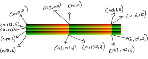
The blue channel is constant everywhere within a cell, and increments by 1 across cells vertically. So the pixel at position (11, 0) will represent the index (0, 131, 0) while the pixel at (12, 0) will represent the index (0, 0, 1). Notice how both the red-index and green-index was reset to 0 when moved down the HaldCLUT image by an entire cell.
The top-left corner extracted from the full identity HaldCLUT. Only the first 3 rows and two columns are shown here (the third column is clipped). Note that the annotations represent the index into the 3d CLUT that pixel represents if the HaldCLUT was instead a normal 3D CLUT. Each cell has the shape (12, 144). When there are two lines in the diagram seemingly coming out from the same pixel, I am trying to show how the represented index changes between adjacent pixels at a cell boundary.
Inspecting the identity HaldCLUT in python reveals the same info:
identity = Image.open("identity.png")
identity = np.asarray(identity)
print("identity HaldCLUT has size: {}".format(identity.shape))
size = round(math.pow(identity.shape[0], 1/3))
print("The CLUT size is {}".format(size))
# The CLUT size is 12
print("clut[0,0] is {}".format(identity[0, 0]))
# clut[0,0] is [0 0 0]
print("clut[0, 100] is {}".format(identity[0, 100]))
# clut[0, 100] is [179   0   0]
print("clut[0, 143] is {}".format(identity[0, 143]))
# We've reached the end of the first row in the first cell
# clut[0, 143] is [255   0   0]
print("clut[0, 144] is {}".format(identity[0, 144]))
# The red channel resets, the green channel increments by 1
# clut[0, 144] is [0 1 0]
print("clut[0, 248] is {}".format(identity[0, 248]))
# clut[0, 248] is [186   1   0]
# Notice how the value in the green channel did not increase. This is normal - we have 256 possible values and only 144 "slots" to keep them. The identity CLUT occasionally skips a
print("clut[0, 432] is {}".format(identity[0, 432]))
# clut[0, 432] is [0 5 0]
# ^ The red got reset, the CLUT skipped more values in the green channel and now maps to 5. This is the peculiarity of this CLUT. A different HaldCLUT (not the identity one) might have had a different value for this green channel step.
print("clut[0, 1727] is {}".format(identity[0, 1727]))
# clut[0, 1727] is [255  19   0]
# This is the last pixel in the first row of the entire image
print("clut[1, 0] is {}".format(identity[1, 0]))
# clut[1, 0] is [ 0 21  0]
# Notice how the value in the green channel "wrapped around" from the previous row
print("clut[1, 144] is {}".format(identity[1, 144]))
# Exercise for the reader: see if you can guess the output correctly 🙂
print("clut[12 0] is {}".format(identity[12, 0]))
print("clut[12 143] is {}".format(identity[12, 143]))
print("clut[12 144] is {}".format(identity[12, 144]))
Applying a HaldCLUT
Now that we’ve understood how a 3D CLUT is sorta encoded in a HaldCLUT png, let’s go ahead and write a method to apply a HaldCLUT to an image:
import math
def apply_hald_clut(hald_img, img):
    hald_w, hald_h = hald_img.size
    clut_size = int(round(math.pow(hald_w, 1/3)))
    # We square the clut_size because a 12-bit HaldCLUT has the same amount of information as a 144-bit 3D CLUT
    scale = (clut_size * clut_size - 1) / 255
    # Convert the PIL image to numpy array
    img = np.asarray(img)
    # We are reshaping to (144 * 144 * 144, 3) - it helps with indexing
    hald_img = np.asarray(hald_img).reshape(clut_size ** 6, 3)
    # Figure out the 3D CLUT indexes corresponding to the pixels in our image
    clut_r = np.rint(img[:, :, 0] * scale).astype(int)
    clut_g = np.rint(img[:, :, 1] * scale).astype(int)
    clut_b = np.rint(img[:, :, 2] * scale).astype(int)
    filtered_image = np.zeros((img.shape))
    # Convert the 3D CLUT indexes into indexes for our HaldCLUT numpy array and copy over the colors to the new image
    filtered_image[:, :] = hald_img[clut_r + clut_size ** 2 * clut_g + clut_size ** 4 * clut_b]
    filtered_image = Image.fromarray(filtered_image.astype('uint8'), 'RGB')
    return filtered_image
Let’s test our method by applying the identity HaldCLUT to our truck – we should get a visually unchanged image back:
Left – the original image, Right – image after apply the “Fuji Velvia 50” HaldCLUT
That worked! You can download more HaldCLUTs from the RawTherapee page. The monochrome (i.e black and white) HaldCLUTs won’t work straight-away because our apply_hald_clut() method expects a hald image with 3 channels (ie reg, green and blue), while the monochrome HaldCLUT images have only 1 channel (the grey value). It won’t be difficult at all to change our method to support monochrome HaldCLUTs – I leave that as an exercise to the reader 😉
Notes and further reading
Remember how we saw that a 2-bit identity CLUT gave us poor results while a 12-bit one almost reproduced our image? That is not necessarily true. Image editing softwares can interpolate between the missing values. For example, this is how PIL apply a 3d CLUT with linear interpolation.
The “Fuji Velvia 50” HaldCLUT that we use is an approximation of Fujifilm’s proprietary velvia film simulation (probably) by Pat Davis
If you want to create your own HaldCLUT, the easiest way would be to open up the identity HaldCLUT png file in an image editing software (e.t.c RawTherapee, Darktable, Adobe Lightroom) and apply global edits to it. For example, if you change the saturation and contrast values to the HaldCLUT png using the image editor, and apply this modified HaldCLUT png (using our python script, or a different image editor – doesn’t matter how) to a different image, the resulting image would have more contrast and saturation. Neat right?
Disclaimer: All I’ve done is write a few config files.
This is for you if:
Your python IDE of choice is PyCharm
You wish you had a command-line replacement for PyCharm on all the places you ssh into
You wish you had access to at least some of the niceties of PyCharm when editing a one-off script, without having to create/import it into a new project.
You are somewhat familiar with vim and can comfortably edit a single file on vim. You also know what a .vimrc is
PyCharm has worked wonderfully well for me, and the only time where I have to use something else is when I ssh into a server to put together a quick script. That something else tends to be vim, and this is an attempt to get vim as close to PyCharm as possible – especially the shortcuts so that I can work on vim the way I work on PyCharm (well, almost). The end result is still a far cry from PyCharm, but it makes navigating a codebase over ssh significantly less painful (at least for me)
But PyCharm can work over ssh
Yeah, but I don’t use PyCharm for one-off scripts. Besides, it pleases me to know that if I can ssh into the server (from an ipad, a phone, or a washing machine), I have an (approximate) IDE I can work on.
List of working approximations
Sorta kinda uses the same colorscheme as PyCharm
Toggles a project navigation sidebar (NERDTree) using alt + 1 . Approximates PyCharm’s Ctrl+1
Comment/uncomment multiple lines using Ctrl+/, just like PyCharm
Autocomplete
Navigate to the definition of a method/variable using Ctrl + Left click or Ctrl + b, just like PyCharm
Jump to the previous location using Alt + - . Approximates PyCharm’s Ctrl + Alt + Left Arrow
Fuzzy search for files using Ctrl + o. Approximates PyCharm’s double shift press
Search the entire code base using Alt + f. Approximates PyCharm’s Ctrl + Shift + f
Edits made in the search results window are reflected on to the underlying file, just like PyCharm
Syntax and linter errors show up as you type, just like PyCharm
If you are editing files that are part of a git repository, there are indicators on the gutter to show added, modified and subtracted lines, just like PyCharm
Pressing F12 brings up a terminal. Approximates PyCharm’s Alt + F12
Code folding using the minus (i.e -) key. Approximates PyCharm’s Ctrl+- and Ctrl + +
Automatic file saves, just like PyCharm
Rename methods/variables and automatically fix imports e.t.c across files, just like PyCharm
Why not just use python-mode?
I simply could not figure out the shortcuts that python-mode used. I thought it would be easier and more flexible if I install and configure the plugins myself.
Prerequisites
vim 8
A Python virtualenv (or a conda environment). There’s some pip install involved, though this is optional
If you need a project-specific .vimrc, see this. If not, everything goes into your ~/.vimrc
Let us begin by being able to see line numbers and some sort of syntax highlighting everywhere. Put these on your .vimrc:
" Some basic stuff
set number
set showmatch
syntax on
imap jj <Esc>
The set showmatch is for highlighting matching parentheses – that’s useful. The last line maps double pressing the j key in insert mode to <Esc> – no more reaching for that far away Escape key using your pinky!
NERDTree for the sidebar
We’ll start our plugin-hoarding with NERDTree. With Vim 8, we can simply copy over a plugin directory to a certain place and Vim would just “pick it up” – there’s no need to use a plugin manager for achieving VimCharm. Create the necessary directory structure and clone NERDTree:
Open some file (any file) on vim and type :NERDTreeToggle – you should see the sidebar. Executing the same command again would close the NERDTree. PyCharm by default opens/closes the sidebar using Ctrl + 1 . However, the terminal (and consequently Vim) cannot differentiate between 1 and Ctrl + 1, so we’ll map this to Alt + 1 instead. Before we do that, we need to determine what characters are sent by the terminal when we press the key combo. Simply run cat without any arguments, and press Alt + 1. You should see something like this:
You would also see that 1 and Ctrl+1 produces the same character on cat – as far as I know, there’s no way around this.
We need to map the character sequence for Alt + 1 to :NERDTreeToggle on our .vimrc:
set <A-1>=^[1
nmap <A-1> :NERDTreeToggle<CR>
Take care not to simply copy paste the character sequence on to your .vimrc! That won’t work. You should open your .vimrc on Vim, go to insert mode, and press Ctrl+v – this would put a caret under your cursor – now press Alt + 1 and it should fill in the necessary characters there. Restart vim, and Alt+1 should now open and close NERDTree.
Making it look like PyCharm
Gruvbox looks like the default PyCharm theme, kinda, so let’s get that:
Ctrl+/ cannot be directly mapped on your .vimrc. So just like before, we insert the correct escaped character sequence into our .vimrc by going into insert mode, pressing Ctrl+v, and then pressing the desired keycombo (Ctrl + / in this case).
" The part after "=" in the below line should be inserted using Ctrl+v while in insert mode and then pressing Ctrl+/
set <F13>=^_
noremap <F13> :call NERDComment(0,"toggle")<CR>

" So that NERDCommenter can automatically decide how to comment a particular filetype
filetype plugin on
We are telling Vim to map the character sequences that Ctrl + / produces to the F13 key, which probably does not exist on your keyboard, and then we map F13 to the appropriate command to toggle comments. Restart Vim, open (or create) a python file and try Ctrl + / while in normal mode – it should comment/uncomment the line.
Autocomplete
Autocomplete on Vim does not feel as “fluid” as on PyCharm – for example, I haven’t managed to get it to work on imports – but it is still besser als nichts. Get jedi-vim:
Restart vim, and Ctrl + space should already be giving you autocomplete suggestions. IMHO, jedi-vim displays too much information (what even is that bar thing that comes up on top?) – all I wanted was a simple autocomplete prompt. Put this on your .vimrc to Make Autocomplete Great Again:
let jedi#show_call_signatures = 0
let jedi#documentation_command = ""
autocmd FileType python setlocal completeopt-=preview
This is something that jedi-vim already does – all we need are some .vimrc entries:
set mouse=a
let g:jedi#goto_command = "<C-LeftMouse>"
map <C-b> <C-LeftMouse>
The above lines enable mouse support on Vim, sets Ctrl + left click as the combination for jedi’s goto command, and then recursively maps Ctrl+b (which is also what PyCharm uses by default) to Ctrl + left click as a keyboard-friendly alternative.
I also prefer the goto command to open a new tab when navigating to a different file. Here’s how to enable that, along with Shift+j and Shift+k to move between tabs:
let g:jedi#use_tabs_not_buffers = 1
nnoremap J :tabp<CR>
nnoremap K :tabn<CR>
Jump to previous location using Alt + minus
If you end up navigating multiple tabs away using Ctrl+b, you can press Ctrl+o repeatedly to jump back to your original position. Press Ctrl+i to go in the other direction. These would come in handy if you have to quickly gg to the beginning of the file to add an import – you can then press Ctrl+o to go back to the line you were editing. I believe in PyCharm the default mappings for this are Ctrl + Alt + Left arrow and Ctrl + Alt + right arrow respectively. I remapped these to Alt + - and Alt + Shift + - (that would be in fact Alt + _ ):
set <A-->=^[-
noremap <A--> <C-O>
set <A-_>=^[_
noremap <A-_> <C-I>
Remember that copy-pasting these won’t work and you will have to enter insert mode and press Ctrl+v and then Alt + -
Fuzzy file search
Fuzzy file search is what PyCharm does when you press the Shift key twice.
By default pressing Ctrl+p should bring up the search prompt. We can’t map this to double shift (as in PyCharm) since vim can’t recognize Shift key presses (unless it’s combined with a printable character). I decided to map this to Ctrl + o instead (“o” for open), though this is not any better than the default setting. On your .vimrc:
let g:ctrlp_map='<C-O>'
let g:ctrlp_cmd='CtrlPMixed'
The second line above specifies that the search should be over files, buffers, tags e.t.c – you may omit it if you do not want buffers to show up on your search. ctrl+t on a search result will open it in a new tab.
Search everywhere and replace
One of the most useful features in PyCharm is the “search in project” dialog that Ctrl + Shift + f brings up. For example, if I delete/rename a hard-coded string literal, this is the dialog that I would bring up to look for all occurrences of that string literal so that I can rename/delete all of them – right from the search window.
Instead of using the built-in vimgrep or making an external call to the ubiquitous grep, we are going to use ack because it excludes annoying things like gitignore and binaries from the search results by default.
git cloneack.vim to ~/.vim/pack/vimcharm/start/ack.vim
We are going to map Alt + F to a python-only smart-cased search with ack. Add these to your .vimrc:
set <A-F>=^[f
nnoremap <A-F> :Ack! -S --python
Remember to Ctr+v and then press Alt+F to get those escaped character sequence right. Also, there is an extra space after the --python. Without it, the search term (eg: “foo”) that you type after pressing Alt+F would end up being “–pythonfoo”.
Restart vim and press Alt+f in a python file, enter your search term, and press enter. The results will be shown in a quick-fix window. Move your cursor to a search result and press enter to jump to that location. Press t to open that location in a new tab. Either of these would shift the focus to the editor. Press ctrl + w twice to shift focus back to the quick-fix window.
I usually use /<pattern> to search within the file, but sometimes it’s useful to do a slightly fancier search. I’ve wired Ctrl+f (the regular PyCharm find-in-this-file) to do a search within the open file:
nnoremap <C-F> :Ack! %<Left><Left>
By default, you cannot make any changes to the contents of the quick-fix window. In Pycharm, the search results are editable and the changes are reflected on the underlying file. We can pull this off using the quickfix-reflector:
That’s it! Now your edits on the search results should be reflected on the underlying files.
Spot syntax and linter errors as you type
The most annoying thing about writing Python on Vim, at least for me, was that the silly syntax errors I make won’t be discovered until I actually try to run my script – PyCharm usually catches these as you type. Let’s set this up on vim using ALE:
You should also have a linter insalled. I use pylint, and a quick pip install pylint does the trick. Restart vim and open a python file, and it should already be linting it as you type. Since ALE works asynchronously, there will be a slight delay (around a second) between you making a mistake and it being flagged on Vim – but in my opinion this is much better than a synchronous linting which freezes Vim, which is why I chose ALE instead of syntastic. However, the default ALE + Pylint combo is too whiny for my taste – I don’t want warnings about how I’m not writing a docstring for every single method; I have this on my .pylintrc:
The above is far from how I would like linter to be configured, but it serves as an initial config. I also do not care for highlighting the offending word in a line – all I want is a non-invasive indication in the gutter. On your .vimrc:
let g:ale_set_highlights = 0
Show lines modified after the previous commit
Put vim-gutter at ~/.vim/pack/vimcharm/start/vim-gutter and restart vim. If you edit a file in a repo (or set up git on your current folder with git init), the modified lines would be marked in the gutter. By default it takes 4 seconds for the appropriate mark to appear on your gutter – let us reduce it by putting this line in the .vimrc:
set updatetime=100
The end result is rather unflattering. ALE and git-gutter does not work well together – git-gutter’s modification marks are drawn over by the linter warnings, and in some-cases ALE ends up marking the wrong line with a warning. This thread suggests that there’s probably a way to get them to work the way I want, but I haven’t invested much time here.
Have a terminal handy
In Vim :term will open a terminal in a split window. Mapping this to F12 is trivial, but we want to hide this terminal (instead of killing it) and bring it back again on pressing F12. I could not get the “hide terminal on F12” part working, but I did figure out how to bring up a hidden terminal if it exists (or create a new terminal if it doesn’t) on pressing F12. Before we write a script for it, let’s go through the motions manually:
Open Vim
Type :term to open a terminal in a split window
Type something on the terminal
Press Ctrl+w and then type :hide to hide our terminal window
To show our hidden terminal, type :sbuffer /bin/bash. This would open in a split window a buffer that has “/bin/bash” in its name. If you use something other than bash, you will have to change this string accordingly.
Here’s a LoadTerminal() Vim script I wrote that would bring up an existing bash buffer if it exists, or create a new one if it doesn’t:
function! LoadTerminal()
    let bnr = bufnr('!/bin/bash')
    if bnr > 0
        :sbuffer !/bin/bash
    else
        :term
    endif
endfunction
Save it as load_terminal.vim at ~/.vim/pack/vimcharm/start and add the following lines to your .vimrc:
The annoying part here is that we can’t map key presses on the terminal window – so you’ll have to press Ctrl + w and type :hide to hide the terminal. Do let me know if you find a way to map this to a keystroke.
Code folding
When you deal with large files, code folding (those tiny “-” signs that you click on PyCharm to collapse an entire class/method) is a godsend. Fortunately vim supports code folding right out of the box and all we need is this on our .vimrc:
set foldmethod=indent
set foldlevelstart=99
nnoremap - za
map _ zM
map + zR
According to our mappings above, there are no folds (i.e every code block is “open”) when we open a file (this is what foldlevelstart specifies). Shift + - (i.e Shift and the minus key) will collapse all blocks, and Shift + + will open all blocks. Use the minus key (i.e -) to toggle collapsing a single fold. You might also want to check out this answer for a quick overview of what’s supported.
Auto save
PyCharm saves the file as you type, sparing you from the hassle of having to press Ctrl+S across multiple tabs. We can get Vim to do this with vim-auto-save. Clone the repo to ~/.vim/pack/vimcharm/start/vim-autosave and add these to your .vimrc to enable auto-save:
let g:auto_save = 1
let g:auto_save_events = ["InsertLeave", "TextChanged"]
A word of caution before we proceed – auto-saving can get quite annoying if enabled globally. I use project-specific vimrcs and use auto-save along with git – so if I accidentally auto-save something that I shouldn’t have, a git diff is all I need to see what went wrong.
Refactor across files
Jedi-vim can do simple renaming, but I wanted to something more powerful. Enter ropevim. You need to pip install rope, ropemode and ropevim. I have a miniconda environment set up, but you can install the packages to your global scope if you want to. We just need one file from the ropevim repo:
We have mapped F6 to the rename operation, and Ctrl+z and Alt + z to undo and redo respectively. Remember not to copy paste the mapping for Alt + z, and press Ctrl+v and then the desired keycombo to enter it in your .vimrc.
Restart Vim, open a python file, and try to rename a variable using F6. You will get prompts to create a new ropevim project – press ‘y’ to create one locally, and then proceed to apply the rename. If you get an import error for ropevim when you start Vim, it’s probably because Vim uses the system python (which is probably a different version than the python in your virtualenv) and you pip-installed rope, ropemode and ropevim to a virtualenv. An alternative would be to do conda install -c conda-forge vim on your anaconda/miniconda env so that the Vim in your env will use the local python (and hence your installed pip packages) instead of the system one.
Final thoughts
If anything this exercise has made be better appreciate the work that the Jetbrains devs have put into their IDEs – all I wanted was a working subset of PyCharm’s basic features and what I got was a rather modest approximation. Do let me know (open an issue on Github?) if you managed to get any closer to PyCharm than this.
TL;DR: Buy a kindle already. Reading multiple books at a time is surprisingly productive.
I now read while I eat. There's a list at the end comparing the amount of reading I got
done before and after I switched to a Kindle
I love smelling books. I also like stacking my books on a table, or on a shelf, so that I can look at them from time to time and be pleased with myself. The stacks also double as cheap room decor – books make the room more me. Then there is the added social benefit of being able to show off to anyone who cares to visit that I have read Thoreau and DDIA*.
* Only half-way through. It has been a year since I purchased the (physical) book. Sigh.
Despite all this, despite arguing with my friends that books are more than just the sum of its parts (late realization: a book has only one “part” that matters – the text) and that smelling a book and then flipping through it is a huge part of the “experience”, I switched to a kindle.
I feel ya, fellow book smellers. Image credits: I got this from a Facebook photo comment :shrugs:
Before you brand me as a traitor and proclaim me unworthy of all the paper books that I have ever smelled, let me assure you that I did not succumb to the dark side easily. I borrowed my dad’s kindle paperwhite and tried it out for an entire month. Then I went out and bought myself a kindle.
The anti-library argument
The number of books I have left partially read has skyrocketed after I switched to the Kindle. And this is a good thing! I have always been a one-book-at-a-time man – I used to carry around the book I was currently reading everywhere, and I would promptly pick up another book after I was done reading the current one. Fast forward to the Kindle era, I find myself reading multiple books at the same time. I had imagined that this would be counter-productive. I’m so happy that I was wrong. The ability to switch to a book on a whim has let me read more than usual since I am reading what I feel like reading now, instead of trying to finish a book that I happened to pick up a week ago out of curiosity. My (unintentional) reading pattern until a few days ago looked like this: Deep Work by Cal Newport during the day, when I find it easy to focus, The Fountainhead for reading on the bed, and The Prince (40% complete) and The rise and fall of the Third Reich (17% complete – this one is a tome) whenever I feel like it. I can confidently say that I would never have made any progress on the last two books if I had stuck to the one book at a time policy that paper books unintentionally forced me to adopt. I would have given up and moved on to the next shiny thing 3 chapters into a history book.
I might never complete reading some of the books that I have on my kindle (looking at you, Third Reich), but that is not the point. In his book Black Swan, Nassim Nicholas Taleb introduces the concept of an anti-library:
The writer Umberto Eco belongs to that small class of scholars who are encyclopedic, insightful, and nondull. He is the owner of a large personal library (containing thirty thousand books), and separates visitors into two categories: those who react with “Wow! Signore professore dottore Eco, what a library you have. How many of these books have you read?” and the others—a very small minority—who get the point is that a private library is not an ego-boosting appendage but a research tool. The library should contain as much of what you do not know as your financial means allow you to put there. You will accumulate more knowledge and more books as you grow older, and the growing number of unread books on the shelves will look at you menacingly. Indeed, the more you know, the larger the rows of unread books. Let us call this collection of unread books an antilibrary.
Replace “unread books” with “partially read books” and you can immediately see how switching to the Kindle has benefitted my anti-library.
The “I now read more” argument
I have been reading on a kindle for about 5 months now, and I do not see myself going back. If there ever was a single compelling advantage that a kindle gave me over paper books, this is it: I read more on a kindle. Much, much more.
I now read while I wait, while I eat, and while I poop. Because the device pleasantly fits into my palm, I can now read while I’m having dinner instead of watching something on YouTube. You maythink that this is not a big deal – but for me, it makes all the difference. Unlike finding time to read, finding time to eat is something that I must do in the interest of self-preservation. Coupling eating with reading is a win-win.
But can’t you just read on your laptop/phone while you eat?
Even if I gloss over the possibility of food on my keyboard, a laptop on the dinner table is just outright inconvenient. Reading on the phone might work. I really do not have a solid reason (apart from the LED screen) as to why I could not bring myself to read on my phone regularly.
I am going to deliberately avoid discussing all the other nice things about using an e-reader. I do find myself taking a lot of notes while I read – something I never used to do with paper books since I couldn’t be bothered to carry around a pen. It is also useful to highlight interesting anecdotes/quotes in a book and then later see them in a compact list. But IMHO these are fringe benefits.
Some raw data
Pre-kindle. List of books I read from September 2017- January 2019 (16 months), in no particular order. This includes both physical books and the few books that I had read on my phone :
Though I am not a “voracious” reader by any stretch of the imagination, you can see that when compared to the pre-kindle rate of 10 books in 16 months, 6 books in 4 months is indeed an improvement. Note that this is considering only the completed books – 17% of “The Rise and Fall of the Third Reich” is as long as some independent books -_-. I admit that the pre-kindle list is likely to be incomplete – I do not remember all the books that I have picked up and left halfway. Nevertheless, the lists should be able to convince you, albeit rather unscientifically, that I read more after I switched to a Kindle
A few years ago, very early into my programming career, I came across a story:
The ceramics teacher announced on opening day that he was dividing the class into two groups. All those on the left side of the studio, he said, would be graded solely on the quantity of work they produced, all those on the right solely on its quality. His procedure was simple: on the final day of class he would bring in his bathroom scales and weigh the work of the “quantity” group: fifty pound of pots rated an “A”, forty pounds a “B”, and so on. Those being graded on “quality”, however, needed to produce only one pot – albeit a perfect one – to get an “A”.
Well, came grading time and a curious fact emerged: the works of highest quality were all produced by the group being graded for quantity. It seems that while the “quantity” group was busily churning out piles of work – and learning from their mistakes – the “quality” group had sat theorizing about perfection, and in the end had little more to show for their efforts than grandiose theories and a pile of dead clay.
This little story has had a tremendous impact on how I approach software engineering as a craft. I was (and still am) convinced that the best way to get better at software engineering is to write more software. I was careful enough to not take the story too seriously – I have always strived to write readable, maintainable code without bugs. However, deep inside my mind was this idea that one day I would be able to write beautiful code without thinking. It would be as effortless to me as breathing. “Refactoring code” would be something left to the apprentice, not something that I, the master who has churned out enough ceramic pots, would be bothered with. I just have to keep making ceramic pots until I get there.
Three years later, I am still very much the apprentice. Rather than programming effortlessly, I have learned to program more deliberately. I have learned (the hard way) to review my code more thoroughly and to refactor it now rather than later. I get pangs of guilt and disappointment every time my pull request has to go through another round of review. I am frustrated when I deliver a feature two days late. As an engineer I want to, above everything else, churn out (the right) features as fast as possible.
Today, I came across an essay that would let me resign from my perpetual struggle to “get faster” at engineering:
I used to have students who bragged to me about how fast they wrote their papers. I would tell them that the great German novelist Thomas Mann said that a writer is someone for whom writing is more difficult than it is for other people. The best writers write much more slowly than everyone else, and the better they are, the slower they write. James Joyce wrote Ulysses, the greatest novel of the 20th century, at the rate of about a hundred words a day
I can strongly relate to this – I would often read and re-read something that I wrote and then I would go back and change it, only to repeat the process again. Though comparing my modest penmanship (keymanship?!) to “the best writers” is outright sacrilegious, even I have in the past noticed that the slower I write, the better I write.
The equivalent in software engineering terms would be to (nothing you did not know before, except for maybe the last point):
Put more thought into the design of your systems
Refactor liberally and lavishly
Test thoroughly
Take your sweet time
As I said, nothing you did not know before. Also, this is almost impossible to pull off when you have realistic business objectives to meet.
But James Joyce probably did not write Ulysses with a publisher breathing down his neck saying “We need to ship this before Christmas!”.
So the secret sauce that makes good code great and the average Joe the next 10x programmer might be this – diligence exercised over a long time.
How does this affect me? Disillusionment. Writing more software does not automatically make you a better programmer. You need the secret sauce, whatever that might be.
Matchertools is my “hello world” project in rust, and I have been chipping away at it slowly and erratically for the past couple of months. You can now find my humble crate here. The crate exposes an API that implements the Gale-Shapley algorithm for the stable marriage problem. Read the wiki. No really, read the linked Wikipedia page. Lloyd Shapley and Alvin Roth won a Nobel prize for this in 2012. Spoiler alert – unlike what the name indicates, the algorithm has little to do with marriages.
This project is so nascent that it is easier for me to list what it does not have:
No documentation
No examples
Shaky integration tests
No code style whatsoever. I haven’t subjected the repo to rustfmt yet (gasp!)
Duct-tape code.
Not nearly enough code comments.
Meta
I had recently adopted a new “philosophy” in life:
Discipline will take you farther than motivation alone ever will
Definitely not me, and more a catch-phrase than philosophy
Most of my side projects do not make it even this far. I go “all-in” for the first couple of days and then my enthusiasm runs out and the project is abandoned before it reaches any meaningful milestone.
But I consciously rate limited myself this time. I had only one aim – work on matchertools every day. I did not really care about the amount of time I spent on the project every day, as long as I made some progress. This also meant that some days I would just read a chapter from the wonderful rust book and that would be it. However, I could not stick to even this plan despite the rather lax constraints – life got in the way. So my aim soon degenerated into “work on matchertools semi-regularly, whenever I can, but be (semi) regular about it“. Thus in two months, I taught myself enough rust to shabbily implement a well-known algorithm. Sarcasm very much intended.
Though I was (am) horrified at the painfully slow pace of the project, the “be slow and semi-regular but keep at it” approach did bear results:
I learned a little rust. I am in love with the language. The documentation is superb!
I produced something, which is far better than my side-project-output in the past 18 months – nothing.
Besides, I have realized that much of what happens around me is unplanned and unpredictable to a larger degree than I had thought. I am currently working on revamping the way I plan things and the way I react when my plans inevitably fail. A little Nassim Nicholas Taleb seems to help, but more on that later.
Learning to play the violin introduced me to western classical music, amateur orchestras, and deliberate practice. Even though I will never seriously pursue music, it was well worth my time.
Some background
I have been taking violin lessons as an adult beginner from 2016 December till now. I have stopped my lessons temporarily since I will be moving to a different city soon. As of January 2019, I am at Suzuki book 3. The decision to pursue violin as an adult might have been influenced by the Carnatic violin lessons I took when I was eleven years old [see sunk cost fallacy].
Also, partly owing to my limited knowledge, I am going to collectively refer to baroque, renaissance and classical music as just “classical music”.
1. Classical music is cool!
I would often come home from a practice session and look up the music we learned that day on Youtube. Though it started as an exercise to get more familiar with the music, I found myself listening to music more actively rather than just letting it play “in the background”. This simple act of being more attentive to what I listen to helped a lot in letting me appreciate classical music.
I was never much interested in the classical genre – most of the pieces I had encountered earlier were simply too long for my short attention span. The lack of an obvious, simple, repeating “chorus” in the genre was something I found hard to come to terms with. However, listening attentively led to the realization that the sophistication and the “cleverness” in the music is something that I could enjoy. My first “aha!” moment was when I stumbled upon the Canon in D. I could see how nuanced the composition was (to my untrained ear), and how each of the violinists seemed to be playing something entirely different yet similar. This was brilliant.
Then there are compositions like the “Moonlight” sonata, which I did not quite like the first time I heard it and now I cannot imagine how I could have not loved it all this while. There is clearly a method to the madness.
My favorite rendition of the Canon in D
2. It is better to progress slowly, but surely.
The vibrato is a technique that every budding violinist hopes to master one day. Six to seven months ago, my vibrato was barely audible – I had to strain my ears to recognize it. Even though I am still a long long way from a respectable vibrato, today I can do some vibrato. A shitty vibrato feels much better than no vibrato.
I did not have to practice particularly hard or long to achieve this. I learn the violin for leisure and is in accordance rather leisurely when it comes to practice. I am happy that though I do not play daily (not a good thing), the 40 minutes of practice I put in 3-4 times a week actually let me (slowly) progress in my lessons. This was new for me. I did not have to work hard to progress – I just had to work somewhat consistently. If I had applied this principle to other things in my life, such as contributing to an open source project or going to the gym, I would have had today a much more braggable resume and much less belly fat.
3. Short, deliberate practice is much better than long hours of unfocused practice
When learning new music, my teacher often tells me that once you learn to play the hardest part the rest becomes very easy. The developer in me resonates with this idea – there is no point in optimizing the rest of your code unless and until you address the bottlenecks. The bottleneck, in my violin lessons, is often fast sections of a composition or parts where I am required to use a new finger position. I would often try to avoid putting in the work and won’t practice the difficult parts separately, partly because playing just the difficult parts is just boring. It is much more pleasurable to attempt the music as a whole and enjoy playing at least a part of the composition, instead of tackling just the difficult parts and consequently sound like a cat being tortured. Inevitably, a few days later, I would realize that I am no closer to playing the music successfully because the difficult parts are holding me back. To make progress, I have always had to prioritize learning the difficult portions.
Some parallels that I can draw to software development include learning new programming paradigms or tackling problems outside your usual domain of expertise. I have recently started reading this wonderful book on mathematics even though I have covered most of the topics as part of my CS bachelors degree. Writing code for the exercises at the end of each chapter is sure to get me out of my comfort zone, and using rust to attempt those exercises will make things more interesting.
4. Use social commitments to your advantage
I performed on a stage for the very first time on October 29, 2018. Even though I played the relatively easier second violin part, the pieces that my teacher chose for the orchestra were beyond my skill level. I had four months to “get my shit together” and “man up” for the big day. Horror-struck by the idea of embarrassing myself in front of a crowd, I started pouring extra time into my practice sessions. Vivaldi’s Summer was a particular pain in the ass – it was simply too fast for me. Eventually, we stopped following the Suzuki books in my personal classes and focused only on being able to play the second violin part of Summer by October.
When the big day came, I was not even nearly ready for that performance. I played a lot of wrong notes and to make things worse, my music stand’s hinge broke and I had to try and read from a stand in the next row. I felt terrible at the end of the day. When I talked to my teacher about how disappointed I was with myself, this was his response:
It does not matter. Do you really think that I do not make mistakes? The final performance was not at all significant compared to what you learned in the months of preparation leading to it.
Raja Singh, The creative school of math and music, New Delhi
The final performance was just an excuse to get the students to punch above their weight class. I must say that it worked – I would not have put in the extra time and effort in the absence of a social commitment. The orchestra also taught me how to follow a conductor, and I could not help but chuckle when I realized that the conductor is just a glorified metronome. Something similar happened when I committed to writing something for my employer’s engineering blog. We were trying to create a brand around the culture we strove to build in the engineering team, and I did not want to do a sloppy job. While I usually invest only a couple of hours into a blog post, this particular one took an entire weekend and went through multiple iterations. The result was head and shoulders above anything I had written till date. Social commitments FTW!
Us performing Mozart’s Symphony No. 25. I’m the tall-ish guy at center-right last row who seems to be barely playing. I need to use more bow *sigh*.
5. It is okay to not like something
My opinion before my introduction to classical music:
Country/Acoustic/Pop > Rock > Hip Hop > Metal > Classical
What I thought my opinion would be after (a mere) 2 years of violin lessons:
Classical music > everything-else > Metal
Unfortunately, such PC master race > console peasantry type comparisons are useless in music. For example, I do not get why people love Chopin. I mean yeah this sounds nice, and I would very much like to claim that I listen to Chopin and thus validate my “superior” taste in music. But the truth is, I like Tarzan and Jane much more than I like Frédéric Chopin. To each his own.